# Workaround for identifying more project IDs. # Used Appeal ID to create unique identifier to group PINs.bor <-read_csv("../Output/borappeals.csv") %>%mutate(project_appellant =paste(project_id, sep ="-", appellant))# modelsummary::datasummary_skim(bor)# Cleaned PIN-Project list after cleaning the commercial valuation dataset found online. # Another temporary work-around until we (maybe) have full keypin list:proj_xwalk <-read_csv("../Output/all_keypins.csv") # all commercial valuation properties but made with not-quite-clean data from commercial valuation dataset on Cook County Data Portal (which was made from combining the Methodology worksheets) # Values are also only the FIRST PASS assessments and do not include appeals or changes in values# Join project IDs to PINs:pin_data <- pin_data %>%left_join(proj_xwalk)# original class_dict variables already in 0_joined data# but I do want the new-ish variables I created to be brought in:class_dict <-read_csv("../Necessary_Files/class_dict_expanded.csv") %>%select(class_code, comparable_props, land_use=Alea_cat)# "Frankfort", "Homer Glen", "Oak Brook", "East Dundee", "University Park", "Bensenville", "Hinsdale", "Roselle", "Deer Park", "Deerfield"cross_county_lines <-c("030440000", "030585000", "030890000", "030320000", "031280000","030080000", "030560000", "031120000", "030280000", "030340000","030150000","030050000", "030180000","030500000", "031210000")pin_data <- pin_data %>%left_join(class_dict, by =c("class"="class_code")) %>%mutate(clean_name =ifelse(is.na(clean_name), "Unincorporated", clean_name)) %>%filter(!agency_num %in% cross_county_lines)# BOR data source shortfall: We only have the data if they appeal!bor_pins <- bor %>%group_by(pin) %>%arrange(desc(tax_year)) %>%summarize(pin =first(pin), # grabs first occurrence of unique PINclass_bor =list(unique(class)),appellant =first(appellant),project_id =first(project_id), timesappealed =n() ) %>%mutate(proj_appellant =paste(project_id, "-", appellant))pin_data <- pin_data %>%left_join(bor_pins, by ="pin")# now do it the other way and comparepin_data <- pin_data %>%mutate( both_ids = project_id,both_ids =ifelse(is.na(both_ids), keypin, both_ids),both_ids =ifelse(is.na(both_ids) &between(class, 300, 899), pin, both_ids))incentive_majorclasses <-c("6", "7A", "7B", "8A", "8B")commercial_classes <-c(401:435, 490, 491, 492, 496:499,500:535,590, 591, 592, 597:599, 700:799,800:835, 891, 892, 897, 899) industrial_classes <-c(480:489,493, 550:589, 593,600:699,850:890, 893 )pin_data <- pin_data %>%mutate(exempt_eav_inTIF =ifelse(in_tif_andpays_revtotif ==1, all_exemptions, 0),untaxable_incent_eav =ifelse(incent_prop ==1, (taxed_av/loa*0.25- taxed_av)*eq_factor, 0),# manually adjust untaxable value of class 239 propertiesuntaxable_value_eav =ifelse(class ==239, eq_av-taxed_eav, untaxable_value_eav),naive_rev_forgone = untaxable_incent_eav * tax_code_rate/100) %>%select(tax_code_num, class, pin, fmv, untaxable_value_fmv, fmv_inTIF, fmv_tif_increment, fmv, tax_bill_total, final_tax_to_dist, final_tax_to_tif, tax_code_rate, taxed_eav, eq_av, av, everything())
Total Value should equal Current Taxable Value + non-Taxable Value where non-Taxable Value = Value in TIF Increment + Reduced Value from Policy Choices where Reduced Value = Tax Exempt Value from Homeowners exemptions or abatements + Reduced Taxable Value from lower levels of assessments due to incentive classifications:
\[\mbox{Total Value = Taxed Value + Untaxable Value}\]
where
\[\mbox{Untaxable Value = TIF Increment + Exemptions + Abatements
+ Reduced Taxable Value from Lower Incentive Class Assessment Ratios}\]
where
\[\mbox{Reduced Taxable Value from Incentive Classification Levels of Assessments}\]\[\mbox{which then equals } {0.25 \ast EAV - \approx0.10 \ast EAV}\]
Cook County Total Value
\[
\mbox{AV = Fair Market Value * Level of Assessment}
\]
Taxed Value refers to what taxing agencies did tax to pay for their levies. We use the portion of the tax bill that does NOT go to TIFs to calculate the portion of the composite levy paid by each PIN and then sum up from there.
\[
\mbox{Final Tax to District} = \mbox{Portion of Levy Paid by PIN} = {\mbox{Tax Code Rate}}*{\mbox{Taxable Value of PIN}}
\]
\[\mbox{Equalized Assessed Value} = {\frac{\mbox{final tax to dist + final tax to TIF}}{\mbox{tax code rate}} + \mbox{Exemptions + Abatements}}\]
Table 8.1: FMV of PINs in Cook County Taxed FMV represents the property value that was actually taxed by local taxing jurisdictions(equal to the amount levied) but converted to FMV. We use the the portion of an individuals tax bill that does NOT go to a TIF to calculate the composite levy for taxing jursidictions.
TO DO Update text in captions automatically based on calculations. Don’t hard code in!
Code
tbl <- cook_sums |>filter(year ==params$year) |>mutate(cty_pct_fmv_both_incent = cty_fmv_incentive / cty_fmv_comandind ,cty_pct_PC_both_incent = cty_PC_withincents / cty_PC_comandind ) |>select(cty_fmv_comandind, #cty_fmv, cty_pct_fmv_both_incent, cty_pct_fmv_incentinTIF, cty_pct_PC_both_incent, cty_PC_comandind, cty_PC_incents_inTIFs, #cty_pct_PC_both_incent_inTIF, cty_pct_fmv_incents_tif_increment) %>%mutate(across(contains("pct_"), scales::percent, accuracy = .01))tbl %>%flextable() %>%align(align ="right") %>%set_header_labels(cty_fmv_comandind ='Com. & Ind. FMV',# cty_fmv = 'Total FMV in Cook',cty_pct_fmv_both_incent ='% of Com. & Ind. FMV w/ Incent.',cty_pct_fmv_incentinTIF ='% of Com. & Ind. FMV w/ Incent. in TIF',cty_pct_fmv_incents_tif_increment ='% of Com. & Ind. FMV in TIF Increment',cty_PC_comandind ='PIN Count',cty_PC_incents_inTIFs ="Incent. PINs in TIF",cty_pct_PC_both_incent ='% of Com. & Ind. PINs w/ Incent.',cty_pct_PC_both_incent_inTIF ='% of Incent. PINs in TIF' ) %>%FitFlextableToPage()
Com. & Ind. FMV
% of Com. & Ind. FMV w/ Incent.
% of Com. & Ind. FMV w/ Incent. in TIF
% of Com. & Ind. PINs w/ Incent.
PIN Count
Incent. PINs in TIF
% of Com. & Ind. FMV in TIF Increment
113,470,082,097
11.25%
41.52%
4.55%
96,275
1,924
26.77%
Table 8.2: Commercial and Industrial PINs in Cook County
11.25% of industrial and commercial PINs (aka "revenue producing PINs") FMV has an incentive classification (4.55% when using PIN counts). Of the PINs that have incentive classification, 41.52% of the FMV is located within a TIF ( NULL 43.9% when using PIN counts).
4.15% of industrial and commercial PINs (aka "revenue producing PINs") FMV has an incentive classification (1.25% when using PIN counts). Of the PINs that have incentive classification, 55.89% of the FMV is located within a TIF ( 40.54% when using PIN counts).
36.7% of industrial PINs FMV has an incentive classification (13.7% when using PIN counts). Of the Industrial PINs that have incentive classification, 35.7% of the FMV is located within a TIF (44% when using PIN counts).
NULL of industrial and commercial PINs (aka "revenue producing PINs") FMV has an incentive classification (NULL when using PIN counts). Of the PINs that have incentive classification, NULL of the FMV is located within a TIF ( NULL when using PIN counts).
Table 8.6: Untaxable AV in Cook County. Taxed AV represents the property value that was actually taxed by local taxing jurisdictions.
Code
cook_sums |>filter(year == params$year) |>select(cty_fmv, cty_fmv_inTIF, cty_fmv_tif_increment, cty_fmv_incentive, cty_fmv_incents_inTIFs, cty_fmv_incents_tif_increment) %>%flextable() %>%set_header_labels(cty_fmv ='Total FMV', cty_fmv_inTIF ='FMV in TIFs',cty_fmv_tif_increment ='TIF Increment FMV' ,cty_fmv_incents_inTIFs ='FMV from Incent. Class in TIF',cty_fmv_incentive ="FMV with Incent.Class.", cty_fmv_incents_tif_increment ='FMV with Incent. Class. in TIF Increment') %>%FitFlextableToPage()
Total FMV
FMV in TIFs
TIF Increment FMV
FMV with Incent.Class.
FMV from Incent. Class in TIF
FMV with Incent. Class. in TIF Increment
605,862,898,192
111,514,487,733
46,298,950,535
12,764,675,273
5,300,523,817
3,417,075,090
Table 8.7: FMV of properties with incentive classifications and TIF increment. Value in TIFs, value within the TIF that can be taxed by local taxing jurisdictions, value of properties that have reduced levels of assessments from incentive classifications, and the value that is both in a TIF and has a reduced LOA.
Taxed value is the amount of value that was actually taxed in order to pay for taxing agencies levies. It includes frozen EAV within an area + taxable EAV for residential properties net exemptions and abatements. It also includes the equalized assessed value of incentive properties at their current, lower assessment ratios. final_tax_to_dist is used to calculate the amount that was collected by local government agencies and then divided by the tax rate to calculate the amount of value that was taxed, or the taxable equalized assessed value (TEAV).
The Taxed Value, when converted to the Fair Market Value (FMV) represents the amount of value that was taxed out of the full FMV available in Cook County.
Untaxable EAV includes homeowner exemptions for 200 level properties, abatements for other property class types, EAV in the TIF increment, and EAV that has been reduced due to incentive classifications.
The Fair Market Value (FMV) is also called the Market Value for
Assessment Purposes and can be calculated from the av /
loa, or the Assessed Value divided by the Level of
Assessment. However, the values used for the level of assessment are an
approximation for incentive properties since we do not have the PIN
level assessment ratios.
Code
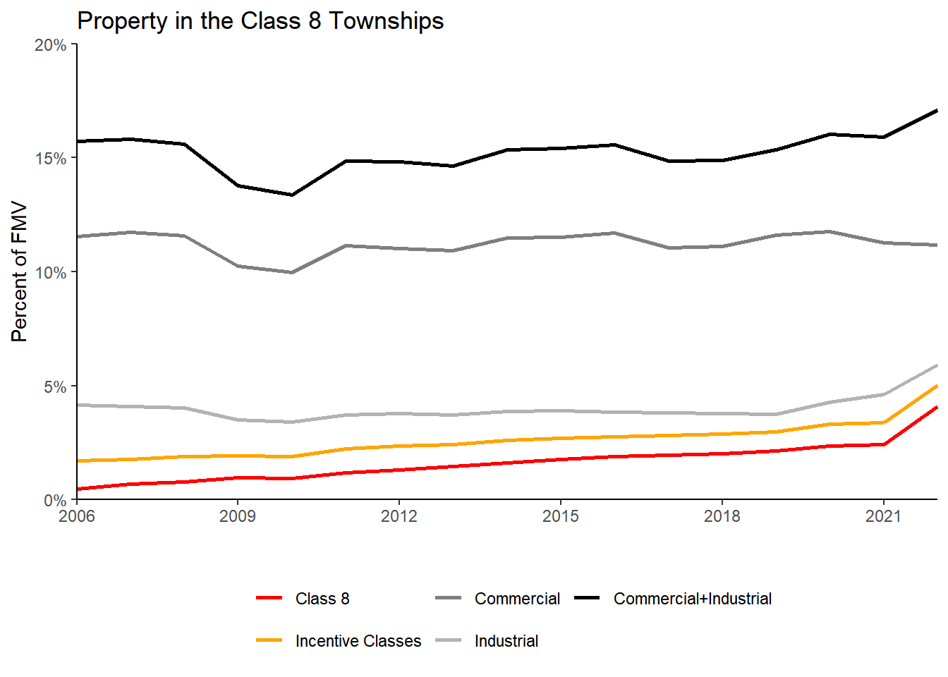
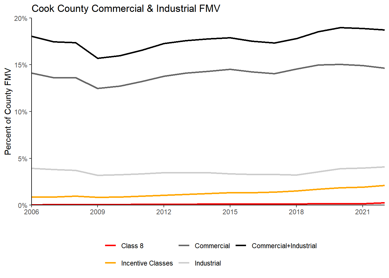
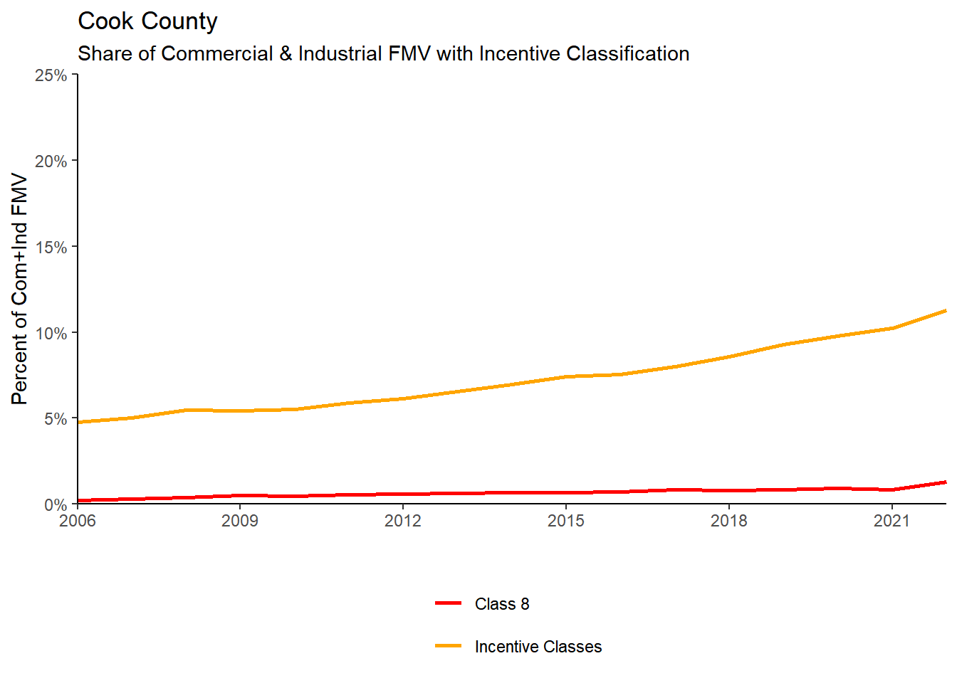
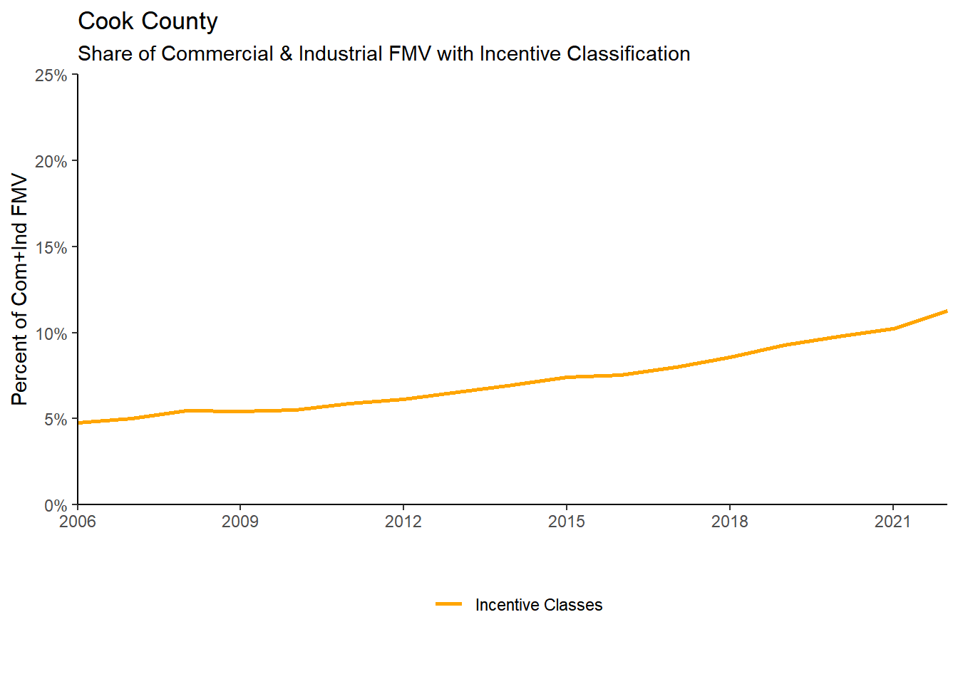
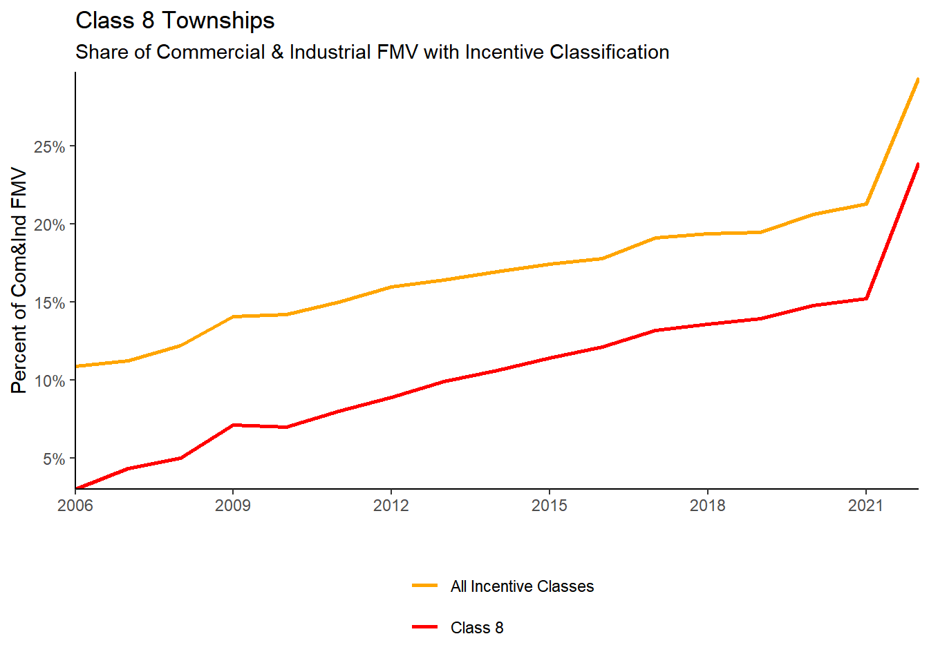
library(tidyverse)options(scipen =999)# Trends in Incentivized FMV as a percent of the base over time## Data prepmuni_MC <-read_csv("../Output/ptaxsim_muni_class_summaries_2006to2023.csv") %>%select(year, clean_name, class, av = muni_c_av)class_dict <-read_csv("../Necessary_Files/class_dict_expanded.csv") %>%select(class = class_code, class_1dig, assess_ratio, incent_prop, land_use=Alea_cat, major_class_code)muni_MC <- muni_MC %>%left_join(class_dict, by =c("class")) %>%filter(class !=0) # drop exempt property types with 0 taxable value#class_8_munis <- read_csv("./Necessary_Files/datarequests_Class8Munis.csv")class_8_munis <-read_csv("../Output/datarequests_Class8Munis.csv")# changed from as.list to as.characterclass_8_munis <-as.character(class_8_munis$clean_name)# class 8 munis - at the year-class levelclass_8_df <-# left_join(muni_MC, class_dict, by = "class") %>% muni_MC %>%filter(clean_name %in% class_8_munis) %>%filter(av !=0) %>%mutate(FMV = av/assess_ratio) %>%group_by(year) %>%mutate(year_tb_tot =sum(FMV)) %>%# tax base for all class 8 munis together, per yearungroup() %>%filter(land_use %in%c("Industrial", "Commercial")) %>%## drops all non-industrial and non-commercial classes to calculate the rest of the totalsgroup_by(year) %>%mutate(year_ind_comm_FMV =sum(FMV)) %>%# total commercial and industrial FMV for all class 8 munis together, per yearungroup() %>%group_by(year, clean_name) %>%mutate(muni_year_ind_comm_FMV =sum(FMV)) %>%# calculates total FMV in each munis each yearungroup() %>%group_by(year, land_use) %>%mutate(cat_year_FMV =sum(FMV)) %>%# calculates FMV within each commercial vs industrial category for each yearungroup() %>%group_by(year, clean_name, class_1dig) %>%# total fmv in class 5, 6, 7, and 8 per munimutate(year_muni_class_FMV =sum(FMV))## Added this for cook level totals:class_8_df_outofCook <- muni_MC %>%# filter(clean_name %in% class_8_munis) %>% ## keep all munis, use for cook county totals.filter(av !=0) %>%mutate(FMV = av/assess_ratio) %>%group_by(year) %>%mutate(year_tb_tot =sum(FMV)) %>%# tax base for all class 8 munis together, per yearungroup() %>%filter(land_use %in%c("Industrial", "Commercial")) %>%## drops all non-industrial and non-commercial classes to calculate the rest of the totalsgroup_by(year) %>%mutate(year_ind_comm_FMV =sum(FMV)) %>%# total commercial and industrial FMV for all class 8 munis together, per yearungroup() %>%group_by(year, clean_name) %>%mutate(muni_year_ind_comm_FMV =sum(FMV)) %>%# calculates total FMV in each munis each yearungroup() %>%group_by(year, land_use) %>%mutate(cat_year_FMV =sum(FMV)) %>%# calculates FMV within each commercial vs industrial category for each yearungroup() %>%group_by(year, clean_name, class_1dig) %>%# total fmv in class 5, 6, 7, and 8 per munimutate(year_muni_class_FMV =sum(FMV))## Class 8 Townships Graph -------------------## Alea Version: ggplot() +geom_line(data = class_8_df %>%group_by(year) %>%summarize(ind_comm_perc =mean(year_ind_comm_FMV/year_tb_tot)), aes(x = year, y = ind_comm_perc, color ="Commercial+Industrial"), lwd =1) +# industrial fmvgeom_line(data = class_8_df %>%filter(land_use =="Industrial") %>%group_by(year) %>%# needed na.rm=TRUE, otherwise it didn't work. perc_industrial was not being calculated without it.summarize(perc_industrial =sum(FMV/year_tb_tot, na.rm=TRUE)), ## added this partaes(x = year, y = perc_industrial, color ="Industrial"), lwd =1) +# commercial fmvgeom_line(data = class_8_df %>%filter(land_use =="Commercial") %>%group_by(year) %>%summarize(perc_commercial =sum(FMV/year_tb_tot, na.rm=TRUE)), ## added this partaes(x = year, y = perc_commercial, color ="Commercial"), lwd =1) +geom_line(data = class_8_df %>%filter(incent_prop =="Incentive") %>%group_by(year) %>%summarise(incent_perc =sum(FMV)/year_tb_tot),aes(x = year, y = incent_perc, color ="Incentive Classes"), lwd =1 ) +geom_line(data = class_8_df %>%# threw error here, missing x and y in aes()filter(class_1dig ==8) %>%group_by(year) %>%summarize(perc_8 =sum(FMV/year_tb_tot)), ## added this partaes(x = year, y = perc_8, color ="Class 8"), lwd =1) +# was missing a + sign heretheme_classic() +scale_x_continuous(name ="", breaks =seq(2006, 2022, by =3), limits =c(2006, 2022), expand =c(0,0)) +scale_y_continuous(name ="Percent of FMV", labels = scales::percent_format(), limits =c(0, 0.20),breaks =seq(0, 0.5, by =0.05), expand =c(0,0)) +scale_color_manual(name ="", values =c("Commercial+Industrial"="black", "Industrial"="gray70", "Commercial"="gray50", "Incentive Classes"="orange", "Class 8"="red" )) +theme(legend.position ="bottom") +labs(title ="Property in the Class 8 Townships") +guides(color =guide_legend(nrow=2, byrow =TRUE))## Percentage out of Cook County ---------------------## Alea Version for Cook Level: ggplot() +# Commercial + Industrial FMV in cookgeom_line(data = class_8_df_outofCook %>%group_by(year) %>%#didn't group by year before?summarize(ind_comm_perc =mean(year_ind_comm_FMV/year_tb_tot)), aes(x = year, y = ind_comm_perc, color ="Commercial+Industrial"), lwd =1) +# incentive class properties in cookgeom_line(data = class_8_df_outofCook %>%filter(incent_prop =="Incentive") %>%group_by(year) %>%summarise(incent_perc =sum(FMV/year_tb_tot)),aes(x = year, y = incent_perc, color ="Incentive Classes"), lwd =1 ) +# FMV with class 8 property class in cook countygeom_line(data = class_8_df_outofCook %>%# threw error here, missing x and y in aes()filter(class_1dig ==8) %>%group_by(year) %>%summarize(perc_8 =sum(FMV/year_tb_tot)), ## added this partaes(x = year, y = perc_8, color ="Class 8"), lwd =1) +# was missing a + sign here# industrial fmv in cook countygeom_line(data = class_8_df_outofCook %>%# threw error here, missing x and y in aes()filter(land_use =="Industrial") %>%group_by(year) %>%# needed na.rm=TRUE, otherwise it didn't work. perc_industrial was not being calculated without it.summarize(perc_industrial =sum(FMV/year_tb_tot, na.rm=TRUE)), ## added this partaes(x = year, y = perc_industrial, color ="Industrial"), lwd =1) +# commercial fmv in cook countygeom_line(data = class_8_df_outofCook %>%# threw error here, missing x and y in aes()filter(land_use =="Commercial") %>%group_by(year) %>%summarize(perc_commercial =sum(FMV/year_tb_tot, na.rm=TRUE)), ## added this partaes(x = year, y = perc_commercial, color ="Commercial"), lwd =1) +# make it pretty:theme_classic() +scale_x_continuous(name ="", breaks =seq(2006, 2022, by =3), limits =c(2006, 2022), expand =c(0,0)) +scale_y_continuous(name ="Percent of County FMV", labels = scales::percent_format(), limits =c(0, 0.20), breaks =seq(0, 0.5, by =0.05), expand =c(0,0)) +scale_color_manual(name ="", values =c("Commercial+Industrial"="black", "Industrial"="gray80", "Commercial"="gray40", "Incentive Classes"="orange", "Class 8"="red")) +theme(legend.position ="bottom") +labs(title="Cook County Commercial & Industrial FMV") +guides(color =guide_legend(nrow=2, byrow =TRUE))## Newest Addition for April 30th Presentation --------------------ggplot() +# incentive class properties in cookgeom_line(data = class_8_df_outofCook %>%filter(incent_prop =="Incentive") %>%group_by(year) %>%summarise(incent_perc =sum(FMV/year_ind_comm_FMV)),aes(x = year, y = incent_perc, color ="Incentive Classes"), lwd =1 ) +# FMV with class 8 property class in cook countygeom_line(data = class_8_df_outofCook %>%filter(class_1dig ==8) %>%group_by(year) %>%summarize(perc_8 =sum(FMV/year_ind_comm_FMV)), aes(x = year, y = perc_8, color ="Class 8"), lwd =1) +# make it pretty:theme_classic() +scale_x_continuous(name ="", breaks =seq(2006, 2022, by =3), limits =c(2006, 2022), expand =c(0,0)) +scale_y_continuous(name ="Percent of Com+Ind FMV", labels = scales::percent_format(), limits =c(0, 0.25), breaks =seq(0, 0.5, by =0.05), expand =c(0,0)) +scale_color_manual(name ="", values =c("Industrial"="gray80", "Commercial"="gray40", "Incentive Classes"="orange", "Class 8"="red")) +theme(legend.position ="bottom") +labs(title="Cook County", subtitle ="Share of Commercial & Industrial FMV with Incentive Classification") +guides(color =guide_legend(nrow=2, byrow =TRUE))## Newest Addition for April 30th Presentation --------------------ggplot() +# incentive class properties in cookgeom_line(data = class_8_df_outofCook %>%filter(incent_prop =="Incentive") %>%group_by(year) %>%summarise(incent_perc =sum(FMV/year_ind_comm_FMV)),aes(x = year, y = incent_perc, color ="Incentive Classes"), lwd =1 ) +# # # FMV with class 8 property class in cook county# geom_line(data = class_8_df_outofCook %>% # filter(class_1dig == 8) %>% # group_by(year) %>%# summarize(perc_8 = sum(FMV/year_ind_comm_FMV)), # aes(x = year, y = perc_8, color = "Class 8"), lwd = 1) + # make it pretty:theme_classic() +scale_x_continuous(name ="", breaks =seq(2006, 2022, by =3), limits =c(2006, 2022), expand =c(0,0)) +scale_y_continuous(name ="Percent of Com+Ind FMV", labels = scales::percent_format(), limits =c(0, 0.25), breaks =seq(0, 0.5, by =0.05), expand =c(0,0)) +scale_color_manual(name ="", values =c("Industrial"="gray80", "Commercial"="gray40", "Incentive Classes"="orange")) +theme(legend.position ="bottom") +labs(title="Cook County", subtitle ="Share of Commercial & Industrial FMV with Incentive Classification") +guides(color =guide_legend(nrow=2, byrow =TRUE))ggplot() +geom_line(data = class_8_df %>%filter(incent_prop =="Incentive") %>%group_by(year) %>%summarise(incent_perc =sum(FMV/year_ind_comm_FMV)),aes(x = year, y = incent_perc, color ="All Incentive Classes"), lwd =1 ) +geom_line(data = class_8_df %>%filter(class_1dig ==8) %>%group_by(year) %>%summarize(perc_8 =sum(FMV/year_ind_comm_FMV)), aes(x = year, y = perc_8, color ="Class 8"), lwd =1) +# make it pretty:theme_classic() +scale_x_continuous(name ="", breaks =seq(2006, 2022, by =3), limits =c(2006, 2022), expand =c(0,0)) +scale_y_continuous(name ="Percent of Com&Ind FMV", labels = scales::percent_format(), # limits = c(0, 0.25), breaks =seq(0, 0.5, by =0.05), expand =c(0,0)) +scale_color_manual(name ="", values =c("Commercial+Industrial"="black", "Industrial"="gray80", "Commercial"="gray40", "All Incentive Classes"="orange", "Class 8"="red")) +theme(legend.position ="bottom") +labs(title="Class 8 Townships", subtitle ="Share of Commercial & Industrial FMV with Incentive Classification") +guides(color =guide_legend(nrow=2, byrow =TRUE))
Municipality Level Stats
Ignore stats for these Municipalities. Simple rounding errors may cause bizarre results for rate changes & other calculations. These municipalities are dropped from summary tables in this website but are included in exported files.
Frankfort has 1 PIN in Cook County
East Dundee has 2
Homer Glen has 3
University Park has 4
Oak Brook, Deer Park, Deerfield, & Bensenville each have less than 75 PINs in Cook County, IL
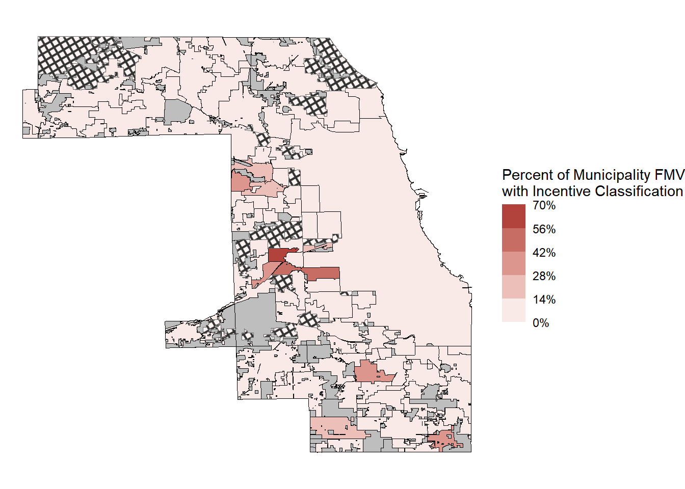
Figure 9.1: Percent of Municipality FMV with Incentive Classification % = FMV from Incentive Class properties / Muni FMV
Code
table2 <- pin_data %>%filter(land_use !="Land") %>%group_by(clean_name, incent_prop) %>%# projects can be counted twice if the project has incentive and normal commercial/industrial prop classes.summarize(pin_count =n(),project_count =n_distinct(keypin), av_adjusted=sum(ifelse(between(class, 600, 899), av*2.5, av)),av=sum(av, na.rm=TRUE),fmv=sum(fmv)) datatable(table2,rownames=FALSE,colnames =c('Municipality'='clean_name', 'Incentivized?'='incent_prop', 'PIN Count'='pin_count', 'Project Count'='project_count', 'Taxable AV'='av')) %>%formatCurrency(c('Taxable AV', 'av_adjusted'), digits =0)
Table 9.4: PINs and value summarized by if the property has an incentive class or not in a municipality. AV Adjusted is the amount of assessed value that could be taxed if the property were assessed at 25% instead of the lower level of assessment of approximately 10%.
Share of Commercial & Industrial FMV with Incentive Classification
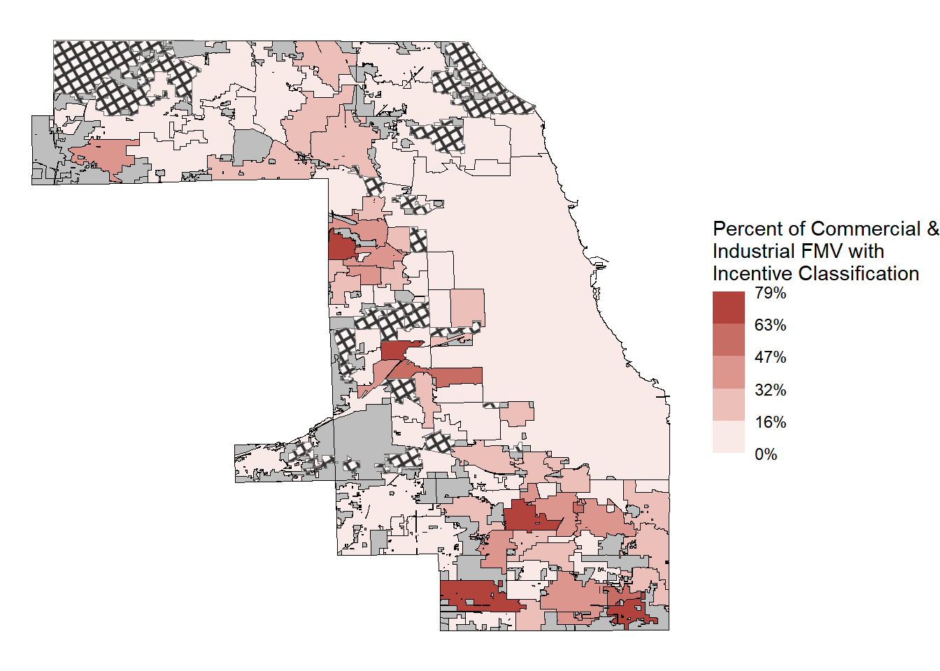
Table 9.5: Municipalities with the largest share of Commercial and Industrial property with incentive classification. Uses tax year 2022 values obtained from PTAXSIM, and levels of assessment from CCAO’s Github. There are 27 municipalities that do not use incentives and have a majority of their taxable EAV within Cook County.
$15 Billion EAV is tax exempt due to homeowners exemptions. All incentive properties combined only have $4 billion EAV that is tax exempt (due to the decreased level of assessment which results in less AV, and therefore, EAV)
Estimates for Revenue Shifted to Non-Incentive Class Properties
Uses old current tax rate and multiplies it by the new taxbase.
Code
pin_data %>%filter(!clean_name %in%c("Frankfort", "Homer Glen", "Oak Brook", "East Dundee","University Park", "Bensenville", "Hinsdale", "Roselle","Deer Park", "Deerfield")) %>%filter(!agency_num %in% cross_county_lines &!is.na(clean_name) & clean_name!="Unincorporated" ) %>%summarize(# for homestead exemptionsmostnaive_forgone_tax_amt_exe =sum(tax_amt_exe), # more accurate but still uses current tax rate instead of recalculated tax rate:forgonerev_from_exemptions =sum(ifelse(class >=200& class <300, (((av*eq_factor) - (taxed_av*eq_factor))) * tax_code_rate/100, 0), na.rm=TRUE),# amount of EAV from taxing an additional 15% of the AV if incentive properties didn't exist# using current tax rate for each property at the tax code levelforgonerev_from_comind_incents =sum(ifelse(class >=600& class <900, (((taxed_av*eq_factor)*0.25- (taxed_av*eq_factor))) * tax_code_rate/100, 0), na.rm=TRUE),forgonerev_commerc_incents =sum(ifelse(class >=600& class <900& class %in% commercial_classes, (((taxed_av*eq_factor)*0.25- (taxed_av*eq_factor))) * tax_code_rate/100, 0), na.rm=TRUE),forgonerev_indust_incents =sum(ifelse(class >=600& class <900& class %in% industrial_classes, (((taxed_av*eq_factor)*0.25- (taxed_av*eq_factor))) * tax_code_rate/100, 0), na.rm=TRUE),# forgonerev_noTIFs = rate_current/100 * ,# TIF increment above the frozen EAVforgonerev_TIFs =sum(fmv_tif_increment * loa * eq_factor*tax_code_rate/100, na.rm=TRUE),# if incentive properties had no tax value (i.e. owners left, or fully tax exempt)# also equal to the current amount collected from incentive propertiesforgonerev_vacant =sum(ifelse(class >=600& class <900, taxed_av*eq_factor * tax_code_rate/100, 0), na.rm =TRUE) )
Change in Composite Property Tax Rate Due to Incentives and other Policy Scenarios
Tables - Difference in Composite Tax Rates
Code
muni_ratechange_sliced <- muni_ratechange %>%# mutate(change_noInc = rate_current - rate_noInc,# change_neither = rate_current - rate_neither,# change_noTIF = rate_current - rate_noTIFs,# change_noExe = rate_current - rate_noExe,# change_vacant = rate_current - rate_vacant,# change_lowest = rate_current - rate_lowest# ) %>%mutate(across(contains("rate_"), round, digits =2))|>select(clean_name, rate_current, rate_noInc, change_noInc) %>%arrange(desc(change_noInc) ) %>%mutate(across(c(rate_current, rate_noInc, change_noInc), round, digits=2)) %>%mutate(change_noInc =abs(round(change_noInc, digits =2)) ) %>%slice(c(1:5, 58:62, 115:119)) muni_ratechange_sliced %>%flextable() %>%border_remove() %>%hline_top() %>%hline(i =c(5,10)) %>%set_header_labels(clean_name ="Municipality", rate_current ="Current Comp.\nTax Rate", rate_noInc ="Tax Rate if No\nIncent. Class.",change_noInc ="Rate Change") %>%bold(i =8) %>%add_footer("There are 26 municipalities that do not use incentives and have a majority of their taxable EAV within Cook County.", top =FALSE) %>%set_table_properties( layout ="autofit")
Municipality
Current Comp. Tax Rate
Tax Rate if No Incent. Class.
Rate Change
Markham
0.28
0.18
0.11
Mc Cook
0.14
0.08
0.06
Sauk Village
0.17
0.12
0.06
Matteson
0.18
0.14
0.04
North Lake
0.12
0.08
0.04
Orland Hills
0.11
0.11
0.00
Rolling Meadows
0.10
0.10
0.00
Midlothian
0.16
0.16
0.00
Richton Park
0.19
0.19
0.00
Niles
0.08
0.08
0.00
Justice
0.12
0.12
0.00
Kenilworth
0.08
0.08
0.00
La Grange Park
0.11
0.11
0.00
Merrionette Park
0.12
0.12
0.00
Morton Grove
0.09
0.09
0.00
Table 10.1: Composite Tax Rate Change from hypothetical scenario of taxing incentive property at 25% of their FMV instead of 10% of their FMV. There are 26 municipalities that do not use incentives and have a majority of their taxable EAV within Cook County.
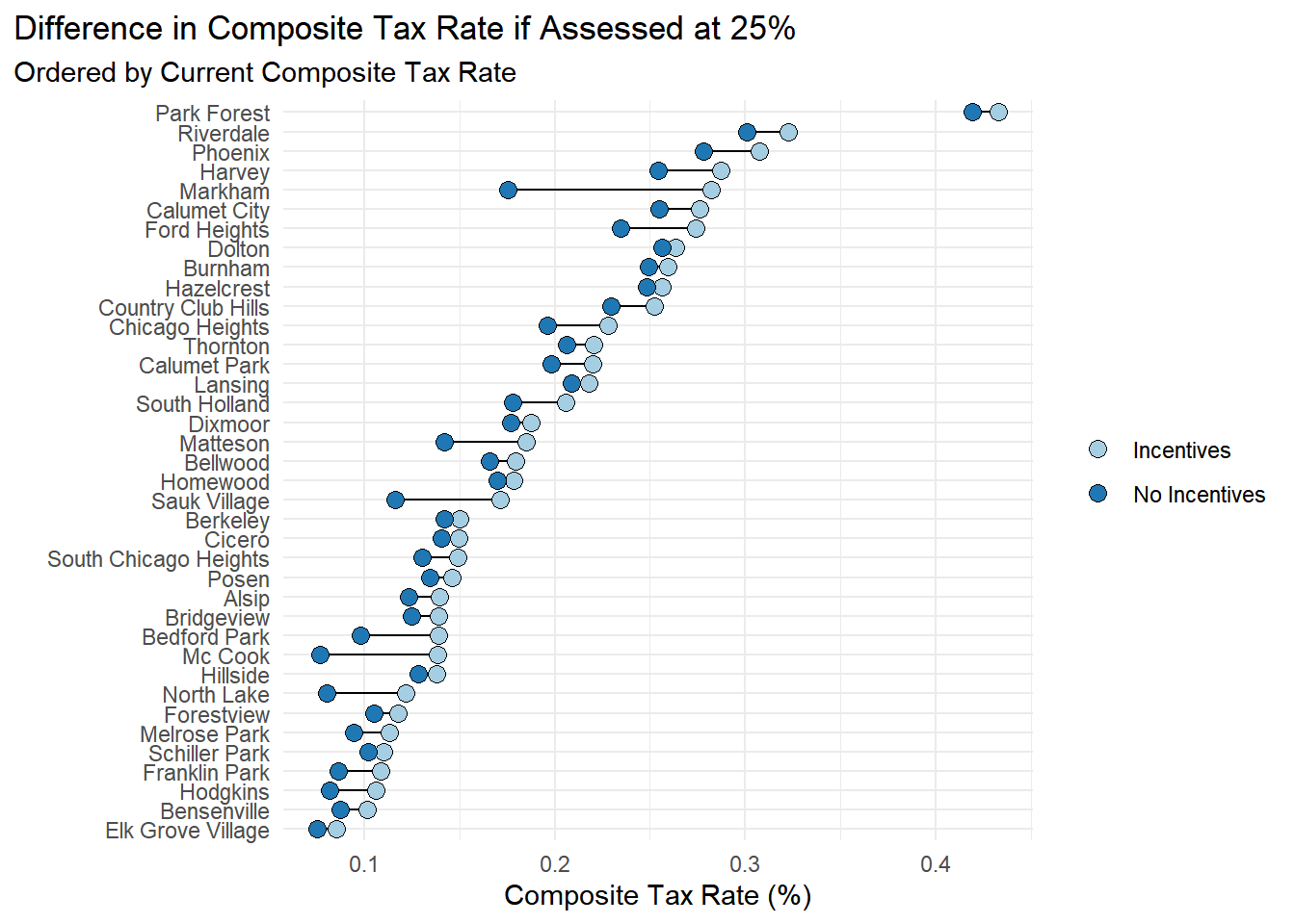
Figure 10.2: Hypothetical change in composite tax rate if all value that currently receives incentive classification became assessed at 25% and exempt EAV from GHE became taxable.
Code
# as a dot graph ## # create order of dotsorder <- muni_ratechange %>%as_tibble() %>%filter(change_noInc >0) %>%arrange(rate_current) %>%select(clean_name, rate_current)# make dot graphmuni_ratechange %>%filter(change_noInc > .007) %>%select(clean_name, rate_current, rate_noInc) %>%distinct() %>%arrange(rate_current) %>%pivot_longer(c("rate_current", "rate_noInc"), names_to ="type", values_to ="tax_rate") %>%inner_join(order) %>%ggplot(aes(x = tax_rate, y=reorder(clean_name, rate_current)))+geom_line(aes(group = clean_name))+geom_point(aes(fill=type), size=3, pch =21, color ="black" )+# scale_color_manual(palette="Blues", # labels = c("Current Rate", "No Incentives")#, # # values = c("#A6CEE3", "#1F78B4" )# )+theme_minimal() +theme( legend.title =element_blank(),plot.title.position ="plot",plot.background =element_rect(fill='transparent', color=NA) #transparent plot bg )+scale_fill_brewer(palette="Paired", labels =c("Incentives", "No Incentives"), direction =1)+labs(title ="Difference in Composite Tax Rate if Assessed at 25%",subtitle ="Ordered by Current Composite Tax Rate", x ="Composite Tax Rate (%)", y ="")
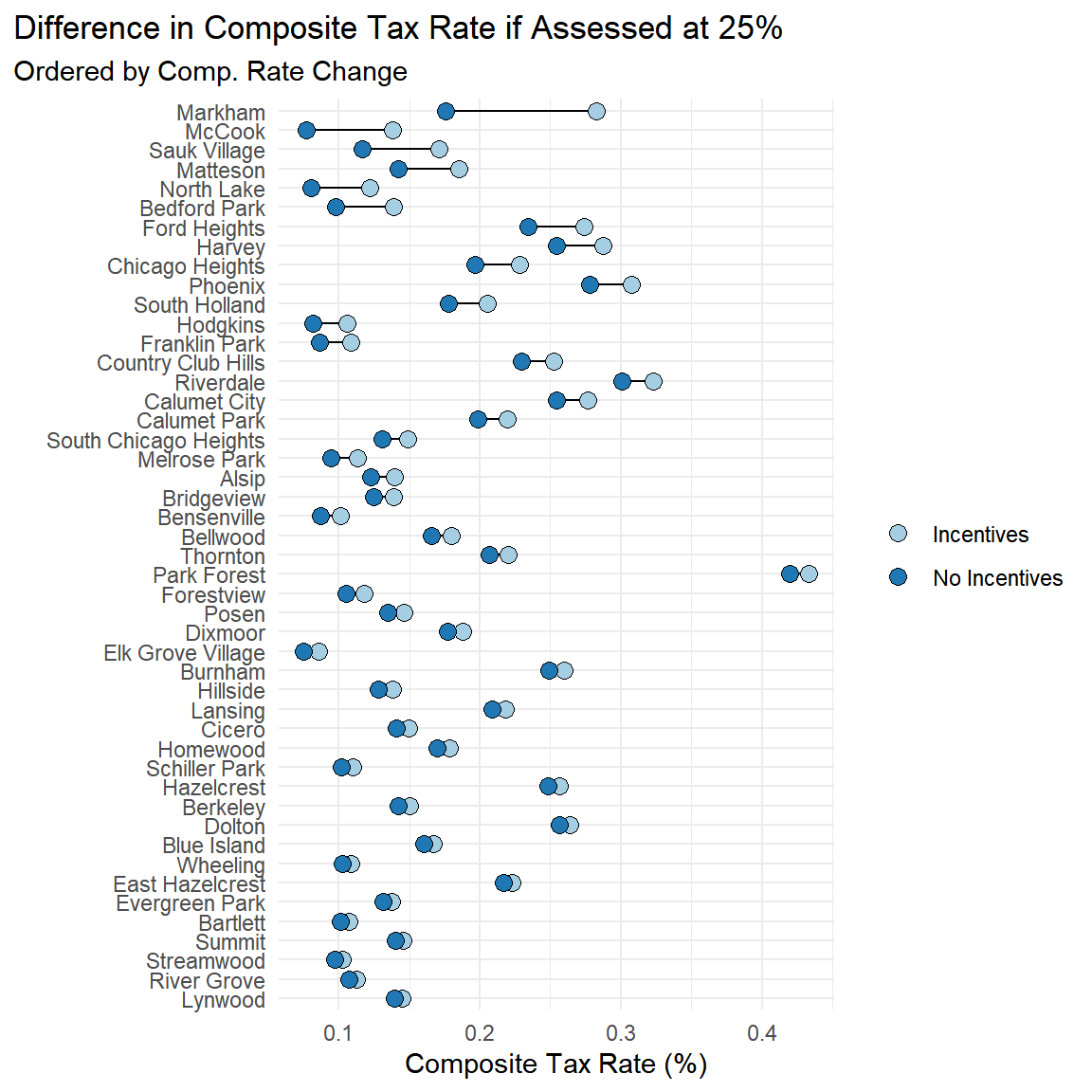
Figure 10.3: Change in tax rate if incentive properties were assessed at 25% of their FMV instead of their reduced level of assessment.
Code
# as a dot graph ## # create order of dotsorder <- muni_ratechange %>%as_tibble() %>%filter(change_noInc >0) %>%arrange(change_noInc) %>%select(clean_name, change_noInc) %>%distinct()# make dot graphmuni_ratechange %>%filter(change_noInc > .005) %>%filter(change_noInc >0) %>%select(clean_name, rate_current, rate_noInc, change_noInc) %>%distinct() %>%pivot_longer(c("rate_current", "rate_noInc"), names_to ="type", values_to ="tax_rate") %>%left_join(order) %>%filter(change_noInc >0 ) %>%mutate(clean_name =if_else(clean_name =="Mc Cook", "McCook", clean_name)) %>%ggplot(aes(x = tax_rate, y=reorder(clean_name, change_noInc)))+geom_line(aes(group = clean_name))+geom_point(aes(fill=type), size=3, pch =21, color ="black" )+theme_minimal() +theme( legend.title =element_blank(),plot.title.position ="plot",plot.background =element_rect(fill='transparent', color=NA) #transparent plot bg )+scale_fill_brewer(palette="Paired", labels =c("Incentives", "No Incentives"), direction =1)+labs(title ="Difference in Composite Tax Rate if Assessed at 25%",subtitle ="Ordered by Comp. Rate Change", x ="Composite Tax Rate (%)", y ="")
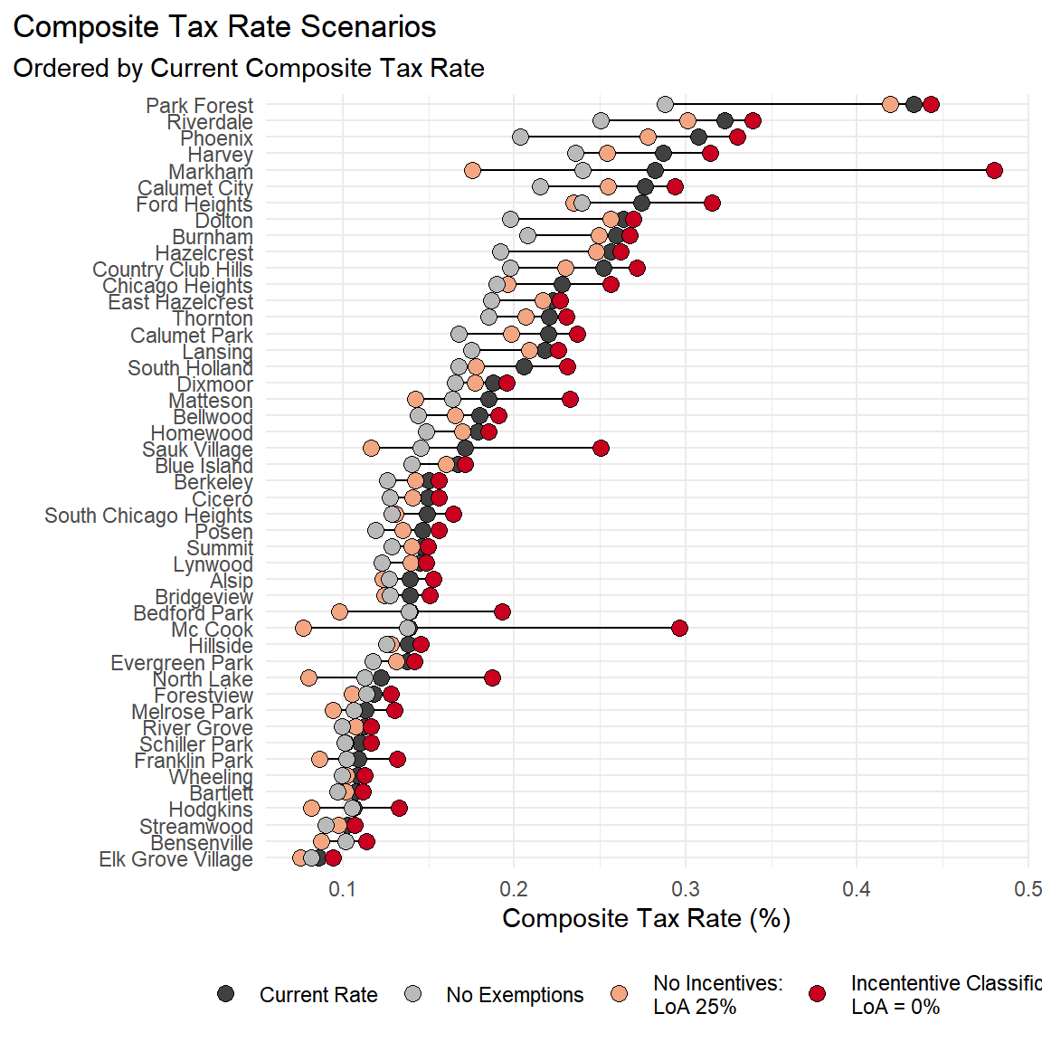
Figure 10.4: Change in Tax Rate from use of Incentives. Ordered by amount of change in the composite tax rate. Only shows municipalities that had more than 1/2 percentage point change in tax rate.
Code
# as a dot graph ## # create order of dotsorder <- muni_ratechange %>%as_tibble() %>%filter(change_noInc >0) %>%arrange(rate_current) %>%select(clean_name, rate_current) %>%distinct()# make dot graphmuni_ratechange %>%filter(change_noInc > .005) %>%select(clean_name, rate_current, rate_noInc, #rate_neither, rate_vacant, rate_noExe) %>%distinct() %>%arrange(rate_current) %>%pivot_longer(c("rate_current", "rate_noInc", "rate_vacant", "rate_noExe"# ,# "rate_neither"), names_to ="type", values_to ="tax_rate") %>%inner_join(order) %>%ggplot(aes(x = tax_rate, y=reorder(clean_name, rate_current)))+geom_line(aes(group = clean_name))+geom_point(aes(fill=type), size=3, pch =21, color ="black" )+theme_minimal() +theme( legend.title =element_blank(),legend.position ="bottom",plot.title.position ="plot",plot.background =element_rect(fill='transparent', color=NA) #transparent plot bg )+scale_fill_brewer(palette ="RdGy",labels =c("Current Rate", # "No Exemps & LoA is 25%","No Exemptions", "No Incentives:\nLoA 25%","Incententive Classification\nLoA = 0%" ), direction =-1)+labs(title ="Composite Tax Rate Scenarios",subtitle ="Ordered by Current Composite Tax Rate", x ="Composite Tax Rate (%)", y ="")
Figure 10.5: Only shows municipalities that had more than 1/2 percentage point change in tax rate.
Code
# as a dot graph ## # create order of dotsorder <- muni_ratechange %>%as_tibble() %>%filter(change_noInc >0) %>%arrange(rate_current) %>%select(clean_name, rate_current) %>%distinct()# make dot graphmuni_ratechange %>%filter(change_noInc >0) %>%select(clean_name, rate_current, rate_noInc, #rate_neither, rate_vacant, rate_noExe) %>%distinct() %>%arrange(rate_current) %>%pivot_longer(c("rate_current", "rate_noInc", "rate_vacant", "rate_noExe"# ,# "rate_neither"), names_to ="type", values_to ="tax_rate") %>%inner_join(order) %>%ggplot(aes(x = tax_rate, y=reorder(clean_name, rate_current)))+geom_line(aes(group = clean_name))+geom_point(aes(fill=type), size=3, pch =21, color ="black" )+theme_minimal() +theme( legend.title =element_blank(),legend.position ="bottom",plot.title.position ="plot",plot.background =element_rect(fill='transparent', color=NA) #transparent plot bg )+scale_fill_brewer(palette ="RdGy",labels =c("Current Rate", # "No Exemps & LoA is 25%","No Exemptions", "No Incentives:\nLoA 25%","Incententive Classification\nLoA = 0%" ), direction =-1)+labs(title ="Composite Tax Rate Scenarios",subtitle ="Ordered by Current Composite Tax Rate", x ="Composite Tax Rate (%)", y ="")
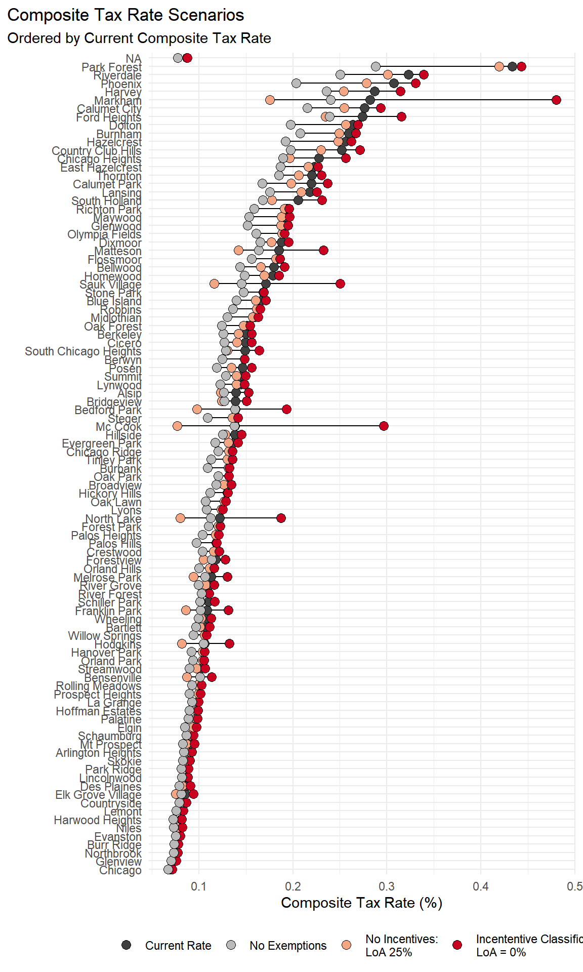
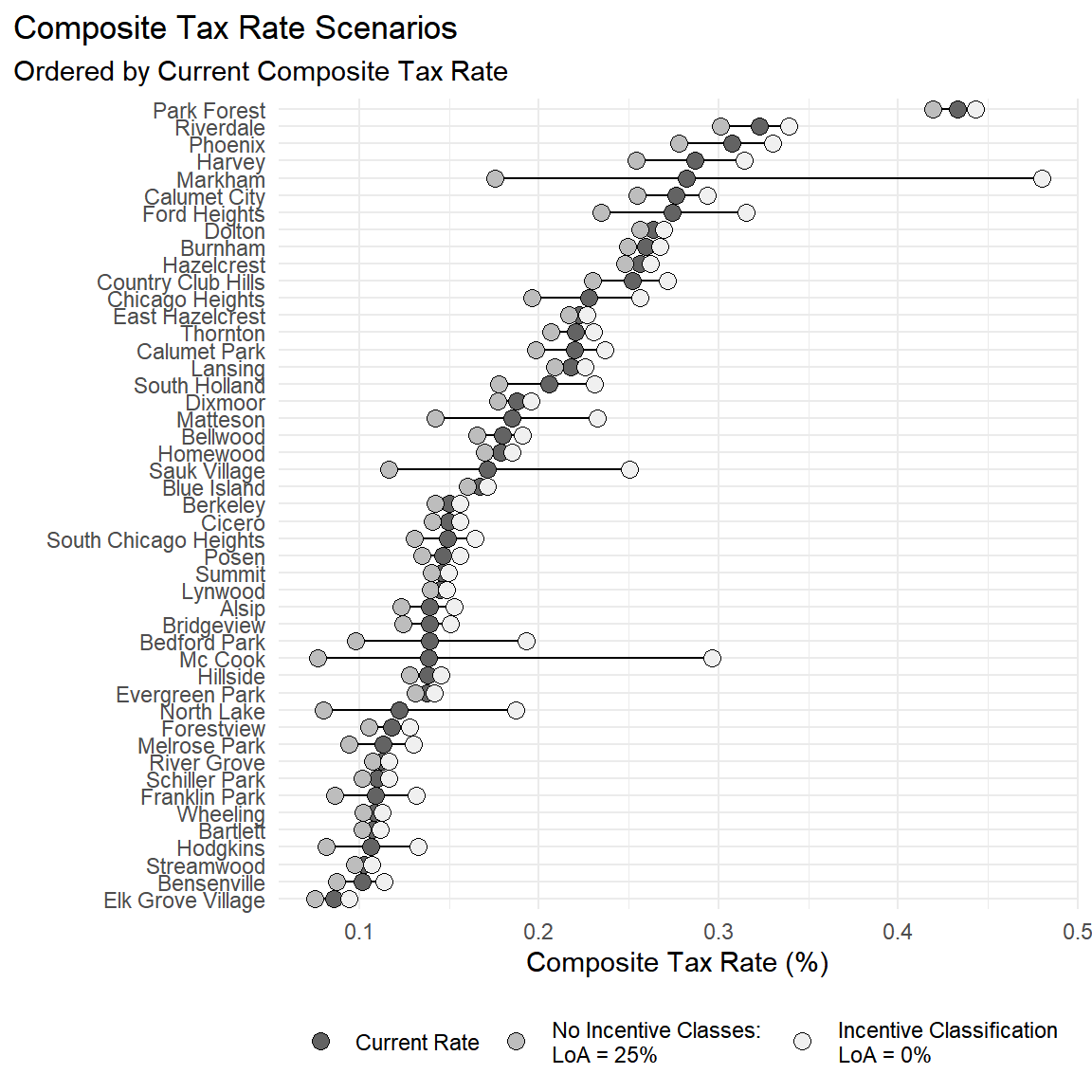
Figure 10.6: Same as figure above but includes all municipalities that had a taxrate change from altering the level of assessment for incentive class properties.
Code
# as a dot graph ## # create order of dotsorder <- muni_ratechange %>%as_tibble() %>%filter(change_noInc > .005) %>%arrange(rate_current) %>%select(clean_name, rate_current) %>%distinct()# make dot graphmuni_ratechange %>%filter(change_noInc > .005) %>%select(clean_name, rate_current, rate_noInc, rate_vacant) %>%distinct() %>%arrange(rate_current) %>%pivot_longer(c("rate_current", "rate_noInc", "rate_vacant" ), names_to ="type", values_to ="tax_rate") %>%inner_join(order) %>%ggplot(aes(x = tax_rate, y=reorder(clean_name, rate_current)))+geom_line(aes(group = clean_name))+geom_point(aes(fill=type), size=3, pch =21, color ="black" )+theme_minimal() +theme( legend.title =element_blank(),legend.position ="bottom",plot.title.position ="plot",plot.background =element_rect(fill='transparent', color=NA) #transparent plot bg )+scale_fill_brewer(palette ="Greys", direction =-1,labels =c("Current Rate", # "No Exemps & LoA is 25%",# "If no Exemptions", "No Incentive Classes: \nLoA = 25%","Incentive Classification\nLoA = 0%" ))+labs(title ="Composite Tax Rate Scenarios",subtitle ="Ordered by Current Composite Tax Rate", x ="Composite Tax Rate (%)", y ="")
Figure 10.7: Only shows municipalities that had more than 1/2 percentage point change in tax rate.
Table 10.2: PIN level tax savings due to incentive classification. Also can be viewed as the shifted tax burden from PINs with incentive classification in 2022 to all other non-incentive PINs. Sorted from largest tax bill savings to smallest bill reduction.
Source Code
---title: "Incentive Classifications"subtitle: "Supporting Content for Cook County C&I Report"format: html: code-fold: true toc: true toc-location: left tbl-cap-location: margin fig-cap-location: margin df-print: pagedparams: year: 2022---```{r setup}#| output: falseknitr::opts_chunk$set(warning = FALSE, message = FALSE)options(scipen = 999)library(tidyverse)library(glue)library(sf)library(DT)library(flextable)nicknames <- readxl::read_excel("../Necessary_Files/muni_shortnames.xlsx")cook_sums <- read_csv("../Output/ptaxsim_cook_level_2006to2023_new.csv") muni_sums <- read_csv("../Output/ptaxsim_muni_level_2006to2023_new.csv")muni_mc_sums <- read_csv("../Output/ptaxsim_muni_MC_2006to2023_new.csv") |> rename_all(~str_replace(., "muni_mc_", ""))muni_cl_sums <- read_csv("../Output/ptaxsim_muni_class_summaries_2006to2023.csv") |> left_join(nicknames)muni_shp <- read_sf("../Necessary_Files/muni_shp.gpkg")knitr::opts_chunk$set(warning = FALSE, message = FALSE)set_flextable_defaults(theme_fun = theme_vanilla, padding = 2, line_spacing = 1, big.mark = ",", )options(DT.options = list())FitFlextableToPage <- function(ft, pgwidth = 6){ ft_out <- ft %>% autofit() ft_out <- width(ft_out, width = dim(ft_out)$widths*pgwidth /(flextable_dim(ft_out)$widths)) return(ft_out)}pin_data <- read_csv(paste0("../Output/Dont_Upload/0_joined_PIN_data_", params$year, "_test.csv"))eq_factor <- read_csv("../Necessary_Files/eq_factor.csv") |> filter(year == params$year) |> select(eq_factor = eq_factor_final) |> as.numeric()``````{r}# Workaround for identifying more project IDs. # Used Appeal ID to create unique identifier to group PINs.bor <-read_csv("../Output/borappeals.csv") %>%mutate(project_appellant =paste(project_id, sep ="-", appellant))# modelsummary::datasummary_skim(bor)# Cleaned PIN-Project list after cleaning the commercial valuation dataset found online. # Another temporary work-around until we (maybe) have full keypin list:proj_xwalk <-read_csv("../Output/all_keypins.csv") # all commercial valuation properties but made with not-quite-clean data from commercial valuation dataset on Cook County Data Portal (which was made from combining the Methodology worksheets) # Values are also only the FIRST PASS assessments and do not include appeals or changes in values# Join project IDs to PINs:pin_data <- pin_data %>%left_join(proj_xwalk)# original class_dict variables already in 0_joined data# but I do want the new-ish variables I created to be brought in:class_dict <-read_csv("../Necessary_Files/class_dict_expanded.csv") %>%select(class_code, comparable_props, land_use=Alea_cat)# "Frankfort", "Homer Glen", "Oak Brook", "East Dundee", "University Park", "Bensenville", "Hinsdale", "Roselle", "Deer Park", "Deerfield"cross_county_lines <-c("030440000", "030585000", "030890000", "030320000", "031280000","030080000", "030560000", "031120000", "030280000", "030340000","030150000","030050000", "030180000","030500000", "031210000")pin_data <- pin_data %>%left_join(class_dict, by =c("class"="class_code")) %>%mutate(clean_name =ifelse(is.na(clean_name), "Unincorporated", clean_name)) %>%filter(!agency_num %in% cross_county_lines)# BOR data source shortfall: We only have the data if they appeal!bor_pins <- bor %>%group_by(pin) %>%arrange(desc(tax_year)) %>%summarize(pin =first(pin), # grabs first occurrence of unique PINclass_bor =list(unique(class)),appellant =first(appellant),project_id =first(project_id), timesappealed =n() ) %>%mutate(proj_appellant =paste(project_id, "-", appellant))pin_data <- pin_data %>%left_join(bor_pins, by ="pin")# now do it the other way and comparepin_data <- pin_data %>%mutate( both_ids = project_id,both_ids =ifelse(is.na(both_ids), keypin, both_ids),both_ids =ifelse(is.na(both_ids) &between(class, 300, 899), pin, both_ids))incentive_majorclasses <-c("6", "7A", "7B", "8A", "8B")commercial_classes <-c(401:435, 490, 491, 492, 496:499,500:535,590, 591, 592, 597:599, 700:799,800:835, 891, 892, 897, 899) industrial_classes <-c(480:489,493, 550:589, 593,600:699,850:890, 893 )pin_data <- pin_data %>%mutate(exempt_eav_inTIF =ifelse(in_tif_andpays_revtotif ==1, all_exemptions, 0),untaxable_incent_eav =ifelse(incent_prop ==1, (taxed_av/loa*0.25- taxed_av)*eq_factor, 0),# manually adjust untaxable value of class 239 propertiesuntaxable_value_eav =ifelse(class ==239, eq_av-taxed_eav, untaxable_value_eav),naive_rev_forgone = untaxable_incent_eav * tax_code_rate/100) %>%select(tax_code_num, class, pin, fmv, untaxable_value_fmv, fmv_inTIF, fmv_tif_increment, fmv, tax_bill_total, final_tax_to_dist, final_tax_to_tif, tax_code_rate, taxed_eav, eq_av, av, everything())```> Total Value should equal Current Taxable Value + non-Taxable Value where non-Taxable Value = Value in TIF Increment + Reduced Value from Policy Choices where Reduced Value = Tax Exempt Value from Homeowners exemptions or abatements + Reduced Taxable Value from lower levels of assessments due to incentive classifications:$$\mbox{Total Value = Taxed Value + Untaxable Value}$$*where*$$\mbox{Untaxable Value = TIF Increment + Exemptions + Abatements + Reduced Taxable Value from Lower Incentive Class Assessment Ratios}$$*where*$$\mbox{Reduced Taxable Value from Incentive Classification Levels of Assessments}$$ $$\mbox{which then equals } {0.25 \ast EAV - \approx0.10 \ast EAV}$$```{r include = FALSE, eval=FALSE}pin_data %>% filter(class == 239) %>% mutate(difference = round(eq_av - (taxed_eav + untaxable_value_eav)), .before = taxed_fmv ) %>% arrange(desc(difference)) %>% head()``````{r include = FALSE}# Are there any properties where the taxed_eav is greater than the original eav value? Nope! yay.pin_data %>% filter(eq_av - taxed_eav < -1)``````{r eval=FALSE, include=FALSE}stopifnot( (pin_data$taxed_eav - pin_data$eq_av <= 10))```# Cook County Total Value$$\mbox{AV = Fair Market Value * Level of Assessment}$$$$\mbox{Tax Rate} = \frac{\mbox{Amount Levied by Taxing Districts}}{\mbox{Taxable Value}}$$> Taxed Value refers to what taxing agencies did tax to pay for their levies. We use the portion of the tax bill that does NOT go to TIFs to calculate the portion of the composite levy paid by each PIN and then sum up from there.$$\mbox{Final Tax to District} = \mbox{Portion of Levy Paid by PIN} = {\mbox{Tax Code Rate}}*{\mbox{Taxable Value of PIN}}$$$$\mbox{Equalized Assessed Value} = {\frac{\mbox{final tax to dist + final tax to TIF}}{\mbox{tax code rate}} + \mbox{Exemptions + Abatements}}$$$$\mbox{Taxed EAV} = {\frac{\sum{final\_tax\_to\_dist}}{\mbox{tax code rate}} + \mbox{Exemptions + Abatements}}$$$$\mbox{Taxed AV} = {\frac{\frac{\sum{final\_tax\_to\_dist}}{\mbox{tax code rate}} + \mbox{Exemptions + Abatements}}{\mbox{county equalizer}}}$$```{r}#| eval: falsetable_cook <- pin_data %>%summarize( cty_PC =n(),cty_PC_industrial =sum(ifelse(class %in% industrial_classes, 1, 0), na.rm =TRUE),cty_PC_commercial =sum(ifelse(class %in% commercial_classes, 1, 0), na.rm =TRUE),cty_PC_com_incent =sum(ifelse(class %in% commercial_classes & incent_prop =="Incentive", 1, 0), na.rm =TRUE),cty_PC_com_incent_inTIF =sum(ifelse(class %in% commercial_classes & incent_prop =="Incentive"& in_tif ==1, 1, 0), na.rm =TRUE),cty_PC_ind_incent =sum(ifelse(class %in% industrial_classes & incent_prop =="Incentive", 1, 0), na.rm =TRUE),cty_PC_ind_incent_inTIF =sum(ifelse(class %in% industrial_classes & incent_prop =="Incentive"& in_tif ==1, 1, 0), na.rm =TRUE),cty_PC_incent =sum(ifelse(incent_prop =="Incentive", 1, 0)),cty_PC_comandind =sum(ifelse((class %in% commercial_classes | class %in% industrial_classes), 1, 0)),cty_PC_comandind_inTIF =sum(ifelse((class %in% commercial_classes | class %in% industrial_classes) & in_tif ==1, 1, 0)),cty_PC_incent_inTIF =sum(ifelse(between(class, 600, 900) & in_tif ==1, 1, 0)),# cty_projects = n_distinct(both_ids), # mostly for industrial and commercial properties. Purposely not assigning keypins to residential properties. cty_fmv_incentive =sum(ifelse(between(class, 600, 900), fmv, 0), na.rm =TRUE),cty_fmv_incent_inTIF =sum(ifelse(between(class, 600, 900) & in_tif ==1, fmv, 0), na.rm =TRUE),cty_fmv_inTIF =sum(fmv_inTIF, na.rm=TRUE),cty_fmv_incents_tif_increment =sum(fmv_incents_tif_increment, na.rm=TRUE),cty_fmv_tif_increment =sum(fmv_tif_increment, na.rm=TRUE),cty_fmv_untaxable_value =sum(untaxable_value_fmv , na.rm=TRUE),cty_fmv =sum(fmv, na.rm=TRUE),cty_fmv_exemptions =sum(all_exemptions/eq_factor/loa, na.rm=TRUE),cty_fmv_abatements =sum((abatements/eq_factor)/loa, na.rm=TRUE),cty_fmv_residential =sum(ifelse(class %in%c(200:399), fmv, 0), na.rm =TRUE),cty_fmv_industrial =sum(ifelse(class %in% industrial_classes, fmv, 0), na.rm =TRUE),cty_fmv_indwithincent =sum(ifelse(class %in% industrial_classes & incent_prop =="Incentive", fmv, 0), na.rm =TRUE),cty_fmv_ind_incent_inTIF=sum(ifelse(class %in% industrial_classes & incent_prop =="Incentive"& in_tif ==1, fmv, 0), na.rm =TRUE),cty_fmv_commercial =sum(ifelse(class %in% commercial_classes, fmv, 0), na.rm =TRUE),cty_fmv_comwithincent =sum(ifelse(class %in% commercial_classes & incent_prop =="Incentive", fmv, 0), na.rm =TRUE),cty_fmv_com_incent_inTIF=sum(ifelse(class %in% commercial_classes & incent_prop =="Incentive"& in_tif ==1, fmv, 0), na.rm =TRUE),cty_fmv_comandind =sum(ifelse(class %in%c(commercial_classes, industrial_classes) , fmv, 0), na.rm =TRUE),cty_levy =sum(final_tax_to_dist),cty_current_rate_avg =mean(tax_code_rate),cty_avg_C2_bill_noexe =mean(ifelse(between(class,200,299) & all_exemptions ==0, (final_tax_to_dist+ final_tax_to_tif), NA), na.rm=TRUE),cty_avg_C2_bill_withexe =mean(ifelse(between(class,200,299) & all_exemptions >0, (final_tax_to_dist+ final_tax_to_tif), NA), na.rm=TRUE),cty_av_taxed =sum(taxed_av, na.rm =TRUE),cty_untaxable_value_av =sum(untaxable_value_av, na.rm=TRUE),cty_av =sum(av),cty_zero_bill =sum(zero_bill, na.rm=TRUE), ) %>%mutate(cty_taxable_value_fmv = cty_fmv - cty_fmv_untaxable_value,cty_pct_fmv_untaxable = cty_fmv_untaxable_value / cty_fmv,# cty_pct_fmv_taxed = cty_fmv_taxed / cty_fmv,cty_pct_fmv_incentinTIF = cty_fmv_incent_inTIF / cty_fmv_incentive,cty_pct_fmv_incents_tif_increment = cty_fmv_incents_tif_increment / cty_fmv_incentive,cty_pct_av_taxed = cty_av_taxed / cty_av,cty_pct_av_untaxable = cty_untaxable_value_av/cty_av,cty_pct_incent_oftotalPC = cty_PC_incent / cty_PC, # incentive pins / all PINscty_pct_incent_ofcomPC = cty_PC_com_incent / cty_PC_commercial, # incentive pins / commercial PINscty_pct_incent_ofindPC = cty_PC_ind_incent / cty_PC_industrial, # incentive pins / commercial PINscty_pct_PC_incent_inTIF = cty_PC_incent_inTIF / cty_PC_incent # count of incentive classes in TIFs / count of incentive Class PINs ) %>%mutate(cty_pct_fmv_both_incent = cty_fmv_comwithincent / cty_fmv_comandind,cty_pct_PC_both_incent = cty_PC_incent / cty_PC_comandind,cty_pct_PC_both_incent_inTIF = cty_PC_incent_inTIF / cty_PC_incent,cty_pct_fmv_both_incent_inTIF = cty_fmv_incent_inTIF / cty_fmv_incentive, )``````{r}#| label: tbl-cooktotals#| tbl-cap: "**FMV of PINs in Cook County** Taxed FMV represents the property value that was actually taxed by local taxing jurisdictions(equal to the amount levied) but converted to FMV. We use the the portion of an individuals tax bill that does NOT go to a TIF to calculate the composite levy for taxing jursidictions."cook_sums %>%filter(year == params$year) |>select(cty_PC, cty_fmv_untaxable_value, cty_fmv, cty_pct_fmv_untaxable) %>%mutate(cty_pct_fmv_untaxable = scales::percent(cty_pct_fmv_untaxable, accuracy =0.01)) %>%flextable() %>%align(align ="right") %>%set_header_labels(cty_PC ='PINs', # cty_projects = "Project IDs", cty_fmv_taxed ='Taxed FMV', cty_fmv_untaxable_value ='FMV not Taxed\nfor Levy',cty_fmv ='Total FMV', cty_pct_fmv_untaxable ='Value not\nTaxed (%)' ) %>%FitFlextableToPage()``````{r add-variable-labels, eval=FALSE, include =FALSE}library(labelled)table_cook <- table_cook %>% set_variable_labels( cty_PC = 'PINs', cty_projects = "Project IDs", cty_fmv = 'Total FMV', cty_fmv_taxed = 'Taxed FMV', cty_fmv_untaxable_value = 'FMV not Taxed\nfor Levy', cty_pct_fmv_untaxable = 'Value not Taxed (%)', cty_fmv_comandind = 'Com. & Ind. FMV', # cty_fmv = 'Total FMV in Cook', cty_pct_fmv_both_incent = '% of Com. & Ind. FMV w/ Incent.', cty_pct_fmv_incentinTIF = '% of Com. & Ind. FMV w/ Incent. in TIF', cty_pct_fmv_incents_tif_increment = '% of Com. & Ind. FMV in TIF Increment', cty_PC_comandind = 'PIN Count', cty_PC_incent_inTIF = "Incent. PINs in TIF", cty_pct_PC_both_incent = '% of Com. & Ind. PINs w/ Incent.', cty_pct_PC_both_incent_inTIF = '% of Incent. PINs in TIF' )```> TO DO Update text in captions automatically based on calculations. Don't hard code in!```{r}#| label: tbl-cooktotals-comandind#| tbl-cap: "**Commercial and Industrial PINs in Cook County**"tbl <- cook_sums |>filter(year ==params$year) |>mutate(cty_pct_fmv_both_incent = cty_fmv_incentive / cty_fmv_comandind ,cty_pct_PC_both_incent = cty_PC_withincents / cty_PC_comandind ) |>select(cty_fmv_comandind, #cty_fmv, cty_pct_fmv_both_incent, cty_pct_fmv_incentinTIF, cty_pct_PC_both_incent, cty_PC_comandind, cty_PC_incents_inTIFs, #cty_pct_PC_both_incent_inTIF, cty_pct_fmv_incents_tif_increment) %>%mutate(across(contains("pct_"), scales::percent, accuracy = .01))tbl %>%flextable() %>%align(align ="right") %>%set_header_labels(cty_fmv_comandind ='Com. & Ind. FMV',# cty_fmv = 'Total FMV in Cook',cty_pct_fmv_both_incent ='% of Com. & Ind. FMV w/ Incent.',cty_pct_fmv_incentinTIF ='% of Com. & Ind. FMV w/ Incent. in TIF',cty_pct_fmv_incents_tif_increment ='% of Com. & Ind. FMV in TIF Increment',cty_PC_comandind ='PIN Count',cty_PC_incents_inTIFs ="Incent. PINs in TIF",cty_pct_PC_both_incent ='% of Com. & Ind. PINs w/ Incent.',cty_pct_PC_both_incent_inTIF ='% of Incent. PINs in TIF' ) %>%FitFlextableToPage()````{r} tbl$cty_pct_fmv_both_incent` of industrial and commercial PINs (aka \"revenue producing PINs\") FMV has an incentive classification (`{r} tbl$cty_pct_PC_both_incent` when using PIN counts). Of the PINs that have incentive classification, `{r} tbl$cty_pct_fmv_incentinTIF` of the FMV is located within a TIF ( `{r} tbl$cty_pct_PC_both_incent_inTIF` 43.9% when using PIN counts).`{r} tbl$cty_pct_fmv_incents_tif_increment` is in TIF Increment.```{r}#| label: tbl-cooktotals-commercial#| tbl-cap: "**Commercial PINs in Cook County**"#table_cook %>% tbl <- cook_sums |>filter(year == params$year) |>mutate(cty_pct_fmv_com_incent = cty_fmv_comwithincent / cty_fmv_commercial,#) |>cty_pct_fmv_com_incent_inTIF = cty_fmv_com_incent_inTIF / cty_fmv_comwithincent,cty_pct_PC_com_incent_inTIF = cty_PC_com_incent_inTIF / cty_PC_com_incent) %>%select(cty_PC_commercial, cty_PC_com_incent, cty_pct_incent_ofcomPC, cty_pct_PC_com_incent_inTIF, cty_fmv_commercial, cty_pct_incent_ofcomPC, cty_pct_fmv_com_incent, cty_pct_fmv_com_incent_inTIF) %>%mutate(across(contains("pct_"), scales::percent, accuracy = .01))tbl %>%flextable() %>%align(align ="right") %>%set_header_labels(cty_fmv_commercial ='Commercial FMV',cty_PC_commercial ='Commercial Pin Count', cty_PC_com_incent ='Com. PIN Count w/ Incent.',cty_pct_incent_ofcomPC ='Com. PINs w/ Incent.',cty_pct_fmv_com_incent ='% of Com. FMV w/ Incent.', cty_pct_fmv_com_incent_inTIF ='% of Com. FMV w/ Incent. in TIF', cty_PC_com_incent_inTIF ="Com. Incent. PINs in TIF", cty_pct_PC_com_incent ='% of Com. PINs w/ Incent.',cty_pct_PC_com_incent_inTIF ='% of Incent. PINs in TIF' ) %>%FitFlextableToPage()````{r} tbl$cty_pct_fmv_com_incent` of industrial and commercial PINs (aka \"revenue producing PINs\") FMV has an incentive classification (`{r} tbl$cty_pct_incent_ofcomPC` when using PIN counts). Of the PINs that have incentive classification, `{r} tbl$cty_pct_fmv_com_incent_inTIF` of the FMV is located within a TIF ( `{r} tbl$cty_pct_PC_com_incent_inTIF` when using PIN counts).`{r} tbl$cty_pct_fmv_com_incents_tif_increment` is in TIF Increment.```{r}#| label: tbl-cooktotals-industrial#| tbl-cap: "**Industrial PINs in Cook County** "cook_sums |>filter(year == params$year) |>mutate(cty_pct_fmv_ind_incent = cty_fmv_indwithincent / cty_fmv_industrial,cty_pct_fmv_ind_incent_inTIF = cty_fmv_ind_incent_inTIF / cty_fmv_indwithincent,cty_pct_PC_ind_incent_inTIF = cty_PC_ind_incent_inTIF / cty_PC_ind_incent) %>%select(cty_PC_industrial, cty_PC_ind_incent, cty_PC_ind_incent_inTIF, cty_pct_incent_ofindPC, cty_pct_fmv_ind_incent_inTIF, cty_pct_PC_ind_incent_inTIF, cty_fmv_industrial, cty_pct_fmv_ind_incent, ) %>%mutate(across(contains("pct_"), scales::percent, accuracy = .01)) %>%flextable() %>%align(align ="right") %>%set_header_labels(cty_fmv_industrial ='Industrial FMV',cty_PC_industrial ='Industrial Pin Count', cty_PC_ind_incent ='Ind. PIN Count w/ Incent.',cty_pct_incent_ofindPC ='Ind. PINs w/ Incent.',cty_pct_fmv_ind_incent ='% of Ind. FMV w/ Incent.', cty_pct_fmv_ind_incent_inTIF ='% of Ind. FMV w/ Incent. in TIF', cty_PC_ind_incent_inTIF ="Ind. Incent. PINs in TIF", cty_pct_PC_ind_incent ='% of Com. PINs w/ Incent.',cty_pct_PC_ind_incent_inTIF ='% of Incent. PINs in TIF' ) %>%FitFlextableToPage()``` 36.7% of industrial PINs FMV has an incentive classification (13.7% when using PIN counts). Of the Industrial PINs that have incentive classification, 35.7% of the FMV is located within a TIF (44% when using PIN counts).`{r} tbl$cty_pct_fmv_ind_incent` of industrial and commercial PINs (aka \"revenue producing PINs\") FMV has an incentive classification (`{r} tbl$cty_pct_incent_ofindPC` when using PIN counts). Of the PINs that have incentive classification, `{r} tbl$cty_pct_fmv_ind_incent_inTIF` of the FMV is located within a TIF ( `{r} tbl$cty_pct_PC_ind_incent_inTIF` when using PIN counts).```{r}#| label: tbl-untaxableFMV-Cook#| tbl-cap: "**Untaxable FMV in Cook County.**"cook_sums |>filter(year == params$year) |>select(cty_fmv, cty_fmv_tif_increment, cty_fmv_exemptions, cty_fmv_abatements, cty_pct_fmv_untaxable ) %>%mutate(across(contains("pct_"), scales::percent, accuracy = .01)) %>%flextable() %>%align(align ="right") %>%set_header_labels(cty_fmv ='Total FMV', cty_fmv_tif_increment ='TIF Increment FMV' ,cty_fmv_exemptions ='Exempt Value: Exemptions',cty_fmv_abatements ='Exempt Value: Abatements',cty_fmv_untaxable_value ='Value not Taxable \nfor Levy',cty_pct_fmv_untaxable ='County FMV not Taxed (%)') %>%FitFlextableToPage()``````{r}#| label: tbl-untaxableAV-Cook#| tbl-cap: "**Untaxable AV in Cook County.** Taxed AV represents the property value that was actually taxed by local taxing jurisdictions."cook_sums |>filter(year == params$year) |>select(cty_av, cty_av_taxed, cty_untaxable_value_av, cty_pct_av_taxed, cty_pct_av_untaxable ) %>%mutate(across(contains("pct_"), scales::percent, accuracy = .01)) %>%flextable() %>%align(align ="right") %>%set_header_labels(cty_av ='Total AV', cty_av_taxed ='Taxed AV' ,cty_untaxable_value_av ='AV Not Taxed',cty_pct_av_taxed ='% Taxed',cty_pct_av_untaxable ='% Not Taxed') %>%FitFlextableToPage()``````{r}#| label: tbl-fmv-intif-withincentive-Cook#| tbl-cap: "**FMV of properties with incentive classifications and TIF increment.** Value in TIFs, value within the TIF that can be taxed by local taxing jurisdictions, value of properties that have reduced levels of assessments from incentive classifications, and the value that is both in a TIF and has a reduced LOA."cook_sums |>filter(year == params$year) |>select(cty_fmv, cty_fmv_inTIF, cty_fmv_tif_increment, cty_fmv_incentive, cty_fmv_incents_inTIFs, cty_fmv_incents_tif_increment) %>%flextable() %>%set_header_labels(cty_fmv ='Total FMV', cty_fmv_inTIF ='FMV in TIFs',cty_fmv_tif_increment ='TIF Increment FMV' ,cty_fmv_incents_inTIFs ='FMV from Incent. Class in TIF',cty_fmv_incentive ="FMV with Incent.Class.", cty_fmv_incents_tif_increment ='FMV with Incent. Class. in TIF Increment') %>%FitFlextableToPage()```**Taxed value** is the amount of value that was actually taxed in order to pay for taxing agencies levies. It includes frozen EAV within an area + taxable EAV for residential properties net exemptions and abatements. It also includes the equalized assessed value of incentive properties at their current, lower assessment ratios. `final_tax_to_dist` is used to calculate the amount that was collected by local government agencies and then divided by the tax rate to calculate the amount of value that was taxed, or the **taxable equalized assessed value (TEAV)**.The Taxed Value, when converted to the Fair Market Value (FMV) represents the amount of value that was taxed out of the full FMV available in Cook County.Untaxable EAV includes homeowner exemptions for 200 level properties, abatements for other property class types, EAV in the TIF increment, and EAV that has been reduced due to incentive classifications.```{r}#| tbl-cap: "The Fair Market Value (FMV) is also called the Market Value for Assessment Purposes and can be calculated from the `av` / `loa`, or the Assessed Value divided by the Level of Assessment. However, the values used for the level of assessment are an approximation for incentive properties since we do not have the PIN level assessment ratios."cty_MC_table <- pin_data %>%group_by(class_group) %>%summarize(cty_MC_PC =n(),cty_MC_projects =n_distinct(both_ids), # mostly for industrial and commercial propertiescty_MC_fmv_incentive =sum(ifelse(incent_prop ==1, fmv, 0), na.rm =TRUE),# cty_MC_fmv_taxed = sum(taxed_fmv, na.rm=TRUE),cty_MC_av_taxed =sum(taxed_av, na.rm=TRUE),cty_MC_fmv_incent_inTIF =sum(ifelse(incent_prop ==1& in_tif ==1, fmv, 0), na.rm =TRUE),cty_MC_fmv_inTIF =sum(fmv_inTIF, na.rm=TRUE),cty_MC_fmv_tif_increment =sum(fmv_tif_increment, na.rm=TRUE),cty_MC_fmv_untaxable_value =sum(untaxable_value_fmv , na.rm=TRUE),cty_MC_fmv =sum(fmv, na.rm=TRUE),cty_MC_fmv_exemptions =sum(all_exemptions/eq_factor/loa, na.rm=TRUE),cty_MC_fmv_abatements =sum(abatements/eq_factor/loa, na.rm=TRUE),cty_MC_cty_zero_bill =sum(zero_bill, na.rm=TRUE),cty_MC_fmv_residential =sum(ifelse(res_prop ==1, fmv, 0), na.rm =TRUE),cty_MC_fmv_industrial =sum(ifelse(class %in% industrial_classes, fmv, 0), na.rm =TRUE),cty_MC_fmv_commercial =sum(ifelse(class %in% commercial_classes, fmv, 0), na.rm =TRUE),cty_MC_levy_paid =sum(final_tax_to_dist),cty_MC_current_rate_avg =mean(tax_code_rate),cty_MC_avg_C2_bill_noexe =mean(ifelse(res_prop ==1& exe_total_adj ==0, (final_tax_to_dist+ final_tax_to_tif), NA), na.rm=TRUE),cty_MC_avg_C2_bill_withexe =mean(ifelse(res_prop ==1& exe_total_adj >0, (final_tax_to_dist+ final_tax_to_tif), NA), na.rm=TRUE), ) %>%mutate( cty_fmv =sum(cty_MC_fmv),pct_cty_MC_fmv_untaxable = cty_MC_fmv_untaxable_value / cty_MC_fmv,# pct_fmv_taxed = cty_MC_fmv_taxed / cty_fmv,pct_MC_levy_paid = cty_MC_levy_paid /sum(cty_MC_levy_paid) )cty_MC_table %>%select(-c(cty_MC_avg_C2_bill_noexe, cty_MC_avg_C2_bill_withexe, cty_MC_fmv_residential, cty_MC_fmv_industrial, cty_MC_fmv_commercial, cty_fmv, #cty_MC_fmv_incent_inTIF ) ) %>%select("Property Type"= class_group, "Homeowner Exempt FMV"= cty_MC_fmv_exemptions,"Abated FMV"= cty_MC_fmv_abatements,"$0 Bill Count"= cty_MC_cty_zero_bill,"$ Levy Paid"= cty_MC_levy_paid,"% of Levy Paid"= pct_MC_levy_paid, "FMV in Major Class"= cty_MC_fmv,"Taxed AV"= cty_MC_av_taxed,"Project Count"= cty_MC_projects,"Avg Composite Tax Rate"= cty_MC_current_rate_avg, everything()) %>%mutate(across(contains("pct_"), scales::percent, accuracy = .01)) %>%flextable() %>%align(align ="right") %>%set_header_labels(cty_MC_PC ='PINs',# projects = "Project IDs", cty_MC_fmv_taxed ='Taxed FMV', cty_MC_fmv_untaxable_value ='Value not Taxable for Levy', cty_MC_fmv_incentive ="FMV with Incent.Class.", cty_MC_fmv_inTIF ='FMV in TIFs', cty_MC_fmv_tif_increment ='TIF Increment FMV',pct_cty_MC_fmv_untaxable ='Value not Taxed (%)', cty_MC_incentive_fmv ='FMV with Incent. Classification',cty_MC_fmv_incent_inTIF ='FMV with Incent. Class. in TIFs' )``````{r}#| layout-ncol: 2#| layout-nrow: 2library(tidyverse)options(scipen =999)# Trends in Incentivized FMV as a percent of the base over time## Data prepmuni_MC <-read_csv("../Output/ptaxsim_muni_class_summaries_2006to2023.csv") %>%select(year, clean_name, class, av = muni_c_av)class_dict <-read_csv("../Necessary_Files/class_dict_expanded.csv") %>%select(class = class_code, class_1dig, assess_ratio, incent_prop, land_use=Alea_cat, major_class_code)muni_MC <- muni_MC %>%left_join(class_dict, by =c("class")) %>%filter(class !=0) # drop exempt property types with 0 taxable value#class_8_munis <- read_csv("./Necessary_Files/datarequests_Class8Munis.csv")class_8_munis <-read_csv("../Output/datarequests_Class8Munis.csv")# changed from as.list to as.characterclass_8_munis <-as.character(class_8_munis$clean_name)# class 8 munis - at the year-class levelclass_8_df <-# left_join(muni_MC, class_dict, by = "class") %>% muni_MC %>%filter(clean_name %in% class_8_munis) %>%filter(av !=0) %>%mutate(FMV = av/assess_ratio) %>%group_by(year) %>%mutate(year_tb_tot =sum(FMV)) %>%# tax base for all class 8 munis together, per yearungroup() %>%filter(land_use %in%c("Industrial", "Commercial")) %>%## drops all non-industrial and non-commercial classes to calculate the rest of the totalsgroup_by(year) %>%mutate(year_ind_comm_FMV =sum(FMV)) %>%# total commercial and industrial FMV for all class 8 munis together, per yearungroup() %>%group_by(year, clean_name) %>%mutate(muni_year_ind_comm_FMV =sum(FMV)) %>%# calculates total FMV in each munis each yearungroup() %>%group_by(year, land_use) %>%mutate(cat_year_FMV =sum(FMV)) %>%# calculates FMV within each commercial vs industrial category for each yearungroup() %>%group_by(year, clean_name, class_1dig) %>%# total fmv in class 5, 6, 7, and 8 per munimutate(year_muni_class_FMV =sum(FMV))## Added this for cook level totals:class_8_df_outofCook <- muni_MC %>%# filter(clean_name %in% class_8_munis) %>% ## keep all munis, use for cook county totals.filter(av !=0) %>%mutate(FMV = av/assess_ratio) %>%group_by(year) %>%mutate(year_tb_tot =sum(FMV)) %>%# tax base for all class 8 munis together, per yearungroup() %>%filter(land_use %in%c("Industrial", "Commercial")) %>%## drops all non-industrial and non-commercial classes to calculate the rest of the totalsgroup_by(year) %>%mutate(year_ind_comm_FMV =sum(FMV)) %>%# total commercial and industrial FMV for all class 8 munis together, per yearungroup() %>%group_by(year, clean_name) %>%mutate(muni_year_ind_comm_FMV =sum(FMV)) %>%# calculates total FMV in each munis each yearungroup() %>%group_by(year, land_use) %>%mutate(cat_year_FMV =sum(FMV)) %>%# calculates FMV within each commercial vs industrial category for each yearungroup() %>%group_by(year, clean_name, class_1dig) %>%# total fmv in class 5, 6, 7, and 8 per munimutate(year_muni_class_FMV =sum(FMV))## Class 8 Townships Graph -------------------## Alea Version: ggplot() +geom_line(data = class_8_df %>%group_by(year) %>%summarize(ind_comm_perc =mean(year_ind_comm_FMV/year_tb_tot)), aes(x = year, y = ind_comm_perc, color ="Commercial+Industrial"), lwd =1) +# industrial fmvgeom_line(data = class_8_df %>%filter(land_use =="Industrial") %>%group_by(year) %>%# needed na.rm=TRUE, otherwise it didn't work. perc_industrial was not being calculated without it.summarize(perc_industrial =sum(FMV/year_tb_tot, na.rm=TRUE)), ## added this partaes(x = year, y = perc_industrial, color ="Industrial"), lwd =1) +# commercial fmvgeom_line(data = class_8_df %>%filter(land_use =="Commercial") %>%group_by(year) %>%summarize(perc_commercial =sum(FMV/year_tb_tot, na.rm=TRUE)), ## added this partaes(x = year, y = perc_commercial, color ="Commercial"), lwd =1) +geom_line(data = class_8_df %>%filter(incent_prop =="Incentive") %>%group_by(year) %>%summarise(incent_perc =sum(FMV)/year_tb_tot),aes(x = year, y = incent_perc, color ="Incentive Classes"), lwd =1 ) +geom_line(data = class_8_df %>%# threw error here, missing x and y in aes()filter(class_1dig ==8) %>%group_by(year) %>%summarize(perc_8 =sum(FMV/year_tb_tot)), ## added this partaes(x = year, y = perc_8, color ="Class 8"), lwd =1) +# was missing a + sign heretheme_classic() +scale_x_continuous(name ="", breaks =seq(2006, 2022, by =3), limits =c(2006, 2022), expand =c(0,0)) +scale_y_continuous(name ="Percent of FMV", labels = scales::percent_format(), limits =c(0, 0.20),breaks =seq(0, 0.5, by =0.05), expand =c(0,0)) +scale_color_manual(name ="", values =c("Commercial+Industrial"="black", "Industrial"="gray70", "Commercial"="gray50", "Incentive Classes"="orange", "Class 8"="red" )) +theme(legend.position ="bottom") +labs(title ="Property in the Class 8 Townships") +guides(color =guide_legend(nrow=2, byrow =TRUE))## Percentage out of Cook County ---------------------## Alea Version for Cook Level: ggplot() +# Commercial + Industrial FMV in cookgeom_line(data = class_8_df_outofCook %>%group_by(year) %>%#didn't group by year before?summarize(ind_comm_perc =mean(year_ind_comm_FMV/year_tb_tot)), aes(x = year, y = ind_comm_perc, color ="Commercial+Industrial"), lwd =1) +# incentive class properties in cookgeom_line(data = class_8_df_outofCook %>%filter(incent_prop =="Incentive") %>%group_by(year) %>%summarise(incent_perc =sum(FMV/year_tb_tot)),aes(x = year, y = incent_perc, color ="Incentive Classes"), lwd =1 ) +# FMV with class 8 property class in cook countygeom_line(data = class_8_df_outofCook %>%# threw error here, missing x and y in aes()filter(class_1dig ==8) %>%group_by(year) %>%summarize(perc_8 =sum(FMV/year_tb_tot)), ## added this partaes(x = year, y = perc_8, color ="Class 8"), lwd =1) +# was missing a + sign here# industrial fmv in cook countygeom_line(data = class_8_df_outofCook %>%# threw error here, missing x and y in aes()filter(land_use =="Industrial") %>%group_by(year) %>%# needed na.rm=TRUE, otherwise it didn't work. perc_industrial was not being calculated without it.summarize(perc_industrial =sum(FMV/year_tb_tot, na.rm=TRUE)), ## added this partaes(x = year, y = perc_industrial, color ="Industrial"), lwd =1) +# commercial fmv in cook countygeom_line(data = class_8_df_outofCook %>%# threw error here, missing x and y in aes()filter(land_use =="Commercial") %>%group_by(year) %>%summarize(perc_commercial =sum(FMV/year_tb_tot, na.rm=TRUE)), ## added this partaes(x = year, y = perc_commercial, color ="Commercial"), lwd =1) +# make it pretty:theme_classic() +scale_x_continuous(name ="", breaks =seq(2006, 2022, by =3), limits =c(2006, 2022), expand =c(0,0)) +scale_y_continuous(name ="Percent of County FMV", labels = scales::percent_format(), limits =c(0, 0.20), breaks =seq(0, 0.5, by =0.05), expand =c(0,0)) +scale_color_manual(name ="", values =c("Commercial+Industrial"="black", "Industrial"="gray80", "Commercial"="gray40", "Incentive Classes"="orange", "Class 8"="red")) +theme(legend.position ="bottom") +labs(title="Cook County Commercial & Industrial FMV") +guides(color =guide_legend(nrow=2, byrow =TRUE))## Newest Addition for April 30th Presentation --------------------ggplot() +# incentive class properties in cookgeom_line(data = class_8_df_outofCook %>%filter(incent_prop =="Incentive") %>%group_by(year) %>%summarise(incent_perc =sum(FMV/year_ind_comm_FMV)),aes(x = year, y = incent_perc, color ="Incentive Classes"), lwd =1 ) +# FMV with class 8 property class in cook countygeom_line(data = class_8_df_outofCook %>%filter(class_1dig ==8) %>%group_by(year) %>%summarize(perc_8 =sum(FMV/year_ind_comm_FMV)), aes(x = year, y = perc_8, color ="Class 8"), lwd =1) +# make it pretty:theme_classic() +scale_x_continuous(name ="", breaks =seq(2006, 2022, by =3), limits =c(2006, 2022), expand =c(0,0)) +scale_y_continuous(name ="Percent of Com+Ind FMV", labels = scales::percent_format(), limits =c(0, 0.25), breaks =seq(0, 0.5, by =0.05), expand =c(0,0)) +scale_color_manual(name ="", values =c("Industrial"="gray80", "Commercial"="gray40", "Incentive Classes"="orange", "Class 8"="red")) +theme(legend.position ="bottom") +labs(title="Cook County", subtitle ="Share of Commercial & Industrial FMV with Incentive Classification") +guides(color =guide_legend(nrow=2, byrow =TRUE))## Newest Addition for April 30th Presentation --------------------ggplot() +# incentive class properties in cookgeom_line(data = class_8_df_outofCook %>%filter(incent_prop =="Incentive") %>%group_by(year) %>%summarise(incent_perc =sum(FMV/year_ind_comm_FMV)),aes(x = year, y = incent_perc, color ="Incentive Classes"), lwd =1 ) +# # # FMV with class 8 property class in cook county# geom_line(data = class_8_df_outofCook %>% # filter(class_1dig == 8) %>% # group_by(year) %>%# summarize(perc_8 = sum(FMV/year_ind_comm_FMV)), # aes(x = year, y = perc_8, color = "Class 8"), lwd = 1) + # make it pretty:theme_classic() +scale_x_continuous(name ="", breaks =seq(2006, 2022, by =3), limits =c(2006, 2022), expand =c(0,0)) +scale_y_continuous(name ="Percent of Com+Ind FMV", labels = scales::percent_format(), limits =c(0, 0.25), breaks =seq(0, 0.5, by =0.05), expand =c(0,0)) +scale_color_manual(name ="", values =c("Industrial"="gray80", "Commercial"="gray40", "Incentive Classes"="orange")) +theme(legend.position ="bottom") +labs(title="Cook County", subtitle ="Share of Commercial & Industrial FMV with Incentive Classification") +guides(color =guide_legend(nrow=2, byrow =TRUE))ggplot() +geom_line(data = class_8_df %>%filter(incent_prop =="Incentive") %>%group_by(year) %>%summarise(incent_perc =sum(FMV/year_ind_comm_FMV)),aes(x = year, y = incent_perc, color ="All Incentive Classes"), lwd =1 ) +geom_line(data = class_8_df %>%filter(class_1dig ==8) %>%group_by(year) %>%summarize(perc_8 =sum(FMV/year_ind_comm_FMV)), aes(x = year, y = perc_8, color ="Class 8"), lwd =1) +# make it pretty:theme_classic() +scale_x_continuous(name ="", breaks =seq(2006, 2022, by =3), limits =c(2006, 2022), expand =c(0,0)) +scale_y_continuous(name ="Percent of Com&Ind FMV", labels = scales::percent_format(), # limits = c(0, 0.25), breaks =seq(0, 0.5, by =0.05), expand =c(0,0)) +scale_color_manual(name ="", values =c("Commercial+Industrial"="black", "Industrial"="gray80", "Commercial"="gray40", "All Incentive Classes"="orange", "Class 8"="red")) +theme(legend.position ="bottom") +labs(title="Class 8 Townships", subtitle ="Share of Commercial & Industrial FMV with Incentive Classification") +guides(color =guide_legend(nrow=2, byrow =TRUE))```# Municipality Level Stats*Ignore stats for these Municipalities. Simple rounding errors may cause bizarre results for rate changes & other calculations. These municipalities are dropped from summary tables in this website but are included in exported files.*- Frankfort has 1 PIN in Cook County- East Dundee has 2- Homer Glen has 3- University Park has 4- Oak Brook, Deer Park, Deerfield, & Bensenville each have less than 75 PINs in Cook County, IL```{r}#| eval: false#| include: falsemunilevel <- pin_data %>%group_by(clean_name) %>%filter(clean_name !="Unincorporated"&!is.na(clean_name)) %>%summarize(muni_exempt_PC =sum(ifelse(class ==0| class =="EX"| class =="RR", 1, 0), na.rm=TRUE),muni_PC_total =n(),muni_PC_residential =sum(ifelse(class %in%c(200:399), 1, 0), na.rm =TRUE),muni_PC_industrial =sum(ifelse(class %in% industrial_classes, 1, 0), na.rm =TRUE),muni_PC_commercial =sum(ifelse(class %in% commercial_classes, 1, 0), na.rm =TRUE),muni_PC_inTIF =sum(in_tif),muni_PC_withincents =sum(ifelse(between(class, 600, 900), 1, 0), na.rm =TRUE),muni_PC_incents_inTIFs =sum(ifelse(between(class, 600, 900) & in_tif ==1, 1, 0), na.rm =TRUE),muni_PC_claimed_exe =sum(ifelse(all_exemptions >0, 1, 0)),# Projects primarily apply to commercial and industrial property.muni_projects =n_distinct(both_ids),muni_fmv_incentive =sum(ifelse(class >=600& class <=900, fmv, 0), na.rm =TRUE),muni_fmv_commerc_incentive =sum(ifelse(class >=600& class <=900& class %in% commercial_classes, fmv, 0), na.rm =TRUE),muni_fmv_indust_incentive =sum(ifelse(class >=600& class <=900& class %in% industrial_classes, fmv, 0), na.rm =TRUE),# muni_fmv_taxed = sum(taxed_fmv, na.rm=TRUE),muni_fmv_inTIF =sum(fmv_inTIF, na.rm=TRUE),muni_fmv_exempt =sum(all_exemptions/eq_factor/loa, na.rm=TRUE),muni_fmv_abated =sum(abatements/eq_factor/loa, na.rm =TRUE),muni_fmv_tif_increment =sum(fmv_tif_increment, na.rm=TRUE),muni_fmv_abates_inTIF =sum(ifelse(between(class, 600, 900) & in_tif ==1& abatements >0 , fmv, 0), na.rm =TRUE),muni_fmv_incents_inTIF =sum(ifelse(between(class, 600, 900) & in_tif ==1, fmv, 0), na.rm =TRUE),muni_fmv_untaxable_value =sum(untaxable_value_fmv , na.rm=TRUE),muni_fmv =sum(fmv, na.rm=TRUE), muni_fmv_residential =sum(ifelse(class %in%c(200:399), fmv, 0), na.rm =TRUE),muni_fmv_industrial =sum(ifelse(class %in% industrial_classes, fmv, 0), na.rm =TRUE),muni_fmv_commercial =sum(ifelse(class %in% commercial_classes, fmv, 0), na.rm =TRUE),muni_zero_bill =sum(zero_bill, na.rm=TRUE),muni_levy =sum(final_tax_to_dist),muni_current_rate_avg =mean(tax_code_rate),muni_eav_taxed =sum(taxed_av*eq_factor), muni_min_TC_rate =min(tax_code_rate),muni_max_TC_rate =max(tax_code_rate),muni_avg_C2_bill_noexe =mean(ifelse(between(class,200,299) & all_exemptions ==0, (final_tax_to_dist + final_tax_to_tif), NA), na.rm=TRUE),muni_avg_C2_bill_withexe =mean(ifelse(between(class,200,299) & all_exemptions >0, (final_tax_to_dist+ final_tax_to_tif), NA), na.rm=TRUE),muni_eav =sum(eav)) %>%mutate(muni_range_TC_rate = muni_max_TC_rate - muni_min_TC_rate,muni_effective_rate = muni_levy / muni_fmv *100, muni_pct_eav_taxed = muni_levy / muni_eav_taxed,# pct_fmv_taxed = muni_fmv_taxed / muni_fmv,pct_fmv_w_incentclass = muni_fmv_incentive / muni_fmv,pct_fmv_indust_incent = muni_fmv_indust_incentive / muni_fmv_industrial,pct_fmv_commerc_incent = muni_fmv_commerc_incentive / muni_fmv_commercial,pct_fmv_inTIF = muni_fmv_inTIF / muni_fmv,pct_fmv_in_tif_increment = muni_fmv_tif_increment / muni_fmv,pct_fmv_untaxable_value = muni_fmv_untaxable_value / muni_fmv,pct_fmv_incents_inTIFs = muni_fmv_incents_inTIF / muni_fmv ) %>%mutate(across(starts_with("muni_fmv_"), round, digits =0)) %>%mutate(across(contains(c("rate", "pct","bill")), round, digits =3) ) %>%ungroup() %>%select(clean_name, everything())```## Frequency of Incentives ### Fair Market Value of Incentive PINs```{r}#| label: tbl-top10industrialincentive-munis#| tbl-cap: "Top 10 Municipalities using Industrial Incentives"landuse_incentshares <- pin_data %>%filter(land_use !="Land") %>%group_by(clean_name, land_use) %>%summarize(pin_count =n(),incent_PC =sum(ifelse(class >=600& class <=900, 1, 0), na.rm=TRUE),fmv_incentive =sum(ifelse(class >=600& class <=900, fmv, 0), na.rm =TRUE),project_count =n_distinct(keypin),fmv_group =sum(fmv, na.rm=TRUE),# av=sum(av) ) %>%mutate(fmv_incentive =ifelse(fmv_incentive ==0, NA, fmv_incentive),pct_incent = fmv_incentive / fmv_group,pct_incent =ifelse(is.na(pct_incent), 0, pct_incent),pct_incent = scales::percent(pct_incent)) indust_top10 <- landuse_incentshares %>%select(clean_name, land_use, fmv_incentive, incent_PC) %>%filter(land_use =="Industrial") %>%arrange(desc(fmv_incentive)) %>%head(10) %>%select(-land_use)indust_top10 %>%flextable() %>%set_header_labels(clean_name ="Municipality", incent_PC ='# of Incent. PINs',fmv_incentive ="FMV from Incentive\nClass Properties") %>%set_table_properties( layout ="autofit", width = .75)``````{r}#| label: tbl-top10commercialincentive-munis#| tbl-cap: "Top 10 Municipalities using Commercial Incentives"commerc_top10 <- landuse_incentshares %>%select(clean_name, land_use, fmv_incentive, incent_PC) %>%filter(land_use =="Commercial") %>%arrange(desc(fmv_incentive)) %>%head(10) %>%select(-land_use)commerc_top10 %>%flextable() %>%#align(align = "right", j = 2:4) %>%set_header_labels(clean_name ="Municipality", incent_PC ='# of Incent. PINs', fmv_incentive ="FMV from Incentive\nClass Properties" ) %>%set_table_properties( layout ="autofit", width = .75)```### Share of Total FMV with Incentive ClassificationCombined Industrial and Commercial FMV with incentive classification divided by total FMV in municipality. Not included in a table in the report.One way of showing areas that have reduced their tax base significantly through the use of incentive classifications. ```{r}table_muni_percentages <- muni_sums %>%filter(year == params$year)|>filter(!clean_name %in%c("Frankfort", "Homer Glen", "Oak Brook", "East Dundee", "University Park", "Bensenville", "Hinsdale", "Roselle", "Deer Park", "Deerfield"))# table_muni_percentages <- munilevel %>% # filter(!clean_name %in% c("Frankfort", "Homer Glen", "Oak Brook", "East Dundee", "University Park", "Bensenville", "Hinsdale", "Roselle", "Deer Park", "Deerfield"))cross_county_line <-c("Frankfort", "Homer Glen", "Oak Brook", "East Dundee", "University Park", "Bensenville", "Hinsdale", "Roselle", "Deer Park", "Deerfield")``````{r}#| label: tbl-muni-percentages#| tbl-cap: "Municipalities with the largest share of FMV property with incentive classification."# table_muni_percentages %>%# select(clean_name, pct_fmv_w_incentclass) |> # arrange(desc(pct_fmv_w_incentclass)) %>%# slice(c(1:10, 56:65, 110:119)) %>%# # #slice(c(1:10, 67:76, 116:125)) %>%# mutate(pct_fmv_w_incentclass = scales::percent(pct_fmv_w_incentclass, digits =1)) %>%# # flextable() %>% # border_remove() %>%# hline_top() %>%# hline(i = c(10,20)) %>%# # set_header_labels(clean_name = "Municipality", pct_fmv_w_incentclass = "% FMV with\nIncent. Class.") %>%# add_header_row(values = c("County Wide", "3.22%"), top = FALSE) %>%# align(j = 2, align = "right") %>%# # set_table_properties( layout = "autofit")table_muni_percentages %>%select(clean_name, pct_fmv_w_incentclass) |>arrange(desc(pct_fmv_w_incentclass)) %>%slice(c(1:5, 69:73, 121:125)) %>%# slice(c(1:5, 58:62, 115:119)) %>%mutate(pct_fmv_w_incentclass = scales::percent(pct_fmv_w_incentclass, digits =2)) %>%flextable() %>%border_remove() %>%hline_top() %>%hline(i =c(5,10)) %>%set_header_labels(clean_name ="Municipality", pct_fmv_w_incentclass ="% FMV") %>%align(j =2, align ="right") %>%align(j=2, align ="right", part ="header") %>%set_table_properties( layout ="autofit")``````{r}library(sf)library(ggpattern)no_incentives <- pin_data %>%# filter(between(class, 600, 899)) %>%group_by(clean_name) %>%summarize(incent_pins =sum(ifelse(between(class, 600, 899), 1, 0))) %>%filter(incent_pins ==0) %>%distinct(clean_name)no_incentives <- no_incentives %>%left_join(muni_shp, by =c("clean_name"="MUNICIPALITY")) # unincorp_areas <- muni_shp %>% filter(!MUNICIPALITY %in% munilevel$clean_name)#anti_join(munilevel, muni_shp, by = c("clean_name" = "MUNICIPALITY"))# unincorp_areas2 <- muni_shp %>% filter(!MUNICIPALITY %in% munilevel$shpfile_name)``````{r}#| label: fig-percentFMVinMunis#| fig-cap: "**Percent of Municipality FMV with Incentive Classification** % = FMV from Incentive Class properties / Muni FMV"#| column: margintable_muni_percentages %>%left_join(nicknames) |>select(clean_name, pct_fmv_w_incentclass, shpfile_name) %>%filter(!is.na(clean_name) & clean_name !="Unincorporated" ) %>%full_join(muni_shp, by =c("shpfile_name"="MUNICIPALITY")) %>%ggplot(aes(fill = pct_fmv_w_incentclass)) +geom_sf(aes(geometry = geom), color ="black") +theme_void() +theme(axis.ticks =element_blank(), axis.text =element_blank())+scale_fill_steps2(high ="brown", low ="black",show.limits=TRUE,nice.breaks=FALSE,na.value="gray",n =4,name ="Percent of Municipality FMV\nwith Incentive Classification",labels = scales::percent) +geom_sf_pattern(data = no_incentives, aes(geometry = geom), pattern ='crosshatch', pattern_spacing =0.015, pattern_density =0.1, fill ="white", alpha = .5, color ='gray40')``````{r}#| label: tbl-muniincentiveuse#| tbl-cap: "PINs and value summarized by if the property has an incentive class or not in a municipality. AV Adjusted is the amount of assessed value that could be taxed if the property were assessed at 25% instead of the lower level of assessment of approximately 10%."table2 <- pin_data %>%filter(land_use !="Land") %>%group_by(clean_name, incent_prop) %>%# projects can be counted twice if the project has incentive and normal commercial/industrial prop classes.summarize(pin_count =n(),project_count =n_distinct(keypin), av_adjusted=sum(ifelse(between(class, 600, 899), av*2.5, av)),av=sum(av, na.rm=TRUE),fmv=sum(fmv)) datatable(table2,rownames=FALSE,colnames =c('Municipality'='clean_name', 'Incentivized?'='incent_prop', 'PIN Count'='pin_count', 'Project Count'='project_count', 'Taxable AV'='av')) %>%formatCurrency(c('Taxable AV', 'av_adjusted'), digits =0)```## Share of Commercial & Industrial FMV with Incentive Classification```{r}#| label: tbl-muni-comind-shareofFMV#| tbl-cap: "Municipalities with the largest share of Commercial and Industrial property with incentive classification. Uses tax year 2022 values obtained from PTAXSIM, and levels of assessment from CCAO's Github. There are 27 municipalities that do not use incentives and have a majority of their taxable EAV within Cook County."muni_incent_share <- pin_data %>%# drop munis mostly outside of Cook and unincorporated PINsfilter(!agency_num %in% cross_county_line &!is.na(clean_name) ) %>%filter(land_use =="Industrial"| land_use =="Commercial") %>%group_by(clean_name, agency_num) %>%summarize(pin_count =n(),incent_PC =sum(ifelse(class >=600& class <900, 1, 0), na.rm=TRUE),fmv_w_incent =sum(ifelse(class >=600& class <900, fmv, 0), na.rm =TRUE),project_count =n_distinct(keypin),fmv_group =sum(fmv, na.rm=TRUE),comind_fmv =sum(fmv, na.rm=TRUE),pins_inTIF =sum(in_tif, na.rm=TRUE)) %>%mutate(fmv_w_incent =ifelse(fmv_w_incent ==0, NA, fmv_w_incent),pct_fmv_w_incent = fmv_w_incent/comind_fmv,pct_fmv_w_incent =ifelse(is.na(pct_fmv_w_incent), 0, pct_fmv_w_incent)) # muni_incentshare_slice <- muni_incent_share %>%# ungroup() %>%# mutate(pct_fmv_w_incentclass = fmv_w_incent/comind_fmv,# pct_fmv_w_incentclass = ifelse(is.na(pct_fmv_w_incentclass), 0, pct_fmv_w_incentclass)) %>%# select(clean_name, pct_fmv_w_incentclass) |> # arrange(desc(pct_fmv_w_incentclass)) %>%# mutate(pct_fmv_w_incentclass = scales::percent(pct_fmv_w_incentclass, accuracy = 0.01) ) %>%# slice(c(1:10, 56:65, 110:119)) # # muni_incentshare_slice %>%# flextable() %>% # border_remove() %>%# hline_top() %>%# hline(i = c(10,20)) %>%# set_header_labels(clean_name = "Municipality", pct_fmv_w_incentclass = "% FMV with\nIncent. Class.") %>%# add_header_row(values = c("County Wide", "3.25%"), top = FALSE) %>%# align(j = 2, align = "right", part = "all") %>%# # add_footer("There are 27 municipalities that do not use incentives and have a majority of their taxable EAV within Cook County.", top = FALSE) %>%# set_table_properties( layout = "autofit")muni_incentshare_slice <- muni_incent_share %>%ungroup() %>%filter(!agency_num %in% cross_county_lines) %>%mutate(pct_fmv_w_incentclass = fmv_w_incent/comind_fmv,pct_fmv_w_incentclass =ifelse(is.na(pct_fmv_w_incentclass), 0, pct_fmv_w_incentclass)) %>%select(clean_name, pct_fmv_w_incentclass) |>arrange(desc(pct_fmv_w_incentclass)) %>%mutate(pct_fmv_w_incentclass = scales::percent(pct_fmv_w_incentclass, accuracy =0.01 ) ) %>%slice(c(1:5, 58:62, 115:119))muni_incentshare_slice %>%flextable() %>%border_remove() %>%align(j =2, align ="right", part ="all") %>%hline_top() %>%hline(i =c(5,10)) %>%set_header_labels(clean_name ="Municipality", pct_fmv_w_incentclass ="% FMV with\nIncent. Class.") %>%#add_header_row(values = c("County Wide", "3.25%"), top = FALSE) %>% align(j = 2, align = "right" ) %>%bold(i =8) %>%set_table_properties( layout ="autofit")``````{r}#| label: fig-shareofcomindFMV#| fig-cap: "Share of Commercial and Industrial FMV that has an incentive property class."muni_incent_share %>%select(clean_name, pct_fmv_w_incent) %>%left_join(nicknames)|>filter(clean_name !="Unincorporated") %>%full_join(muni_shp, by =c("shpfile_name"="MUNICIPALITY")) %>%ggplot(aes(fill = pct_fmv_w_incent)) +geom_sf(aes(geometry = geom), color ="black") +theme_void() +theme(axis.ticks =element_blank(), axis.text =element_blank())+scale_fill_steps2(high ="brown", low ="black",show.limits=TRUE,nice.breaks=FALSE,na.value="gray",n =4,name ="Percent of Commercial &\nIndustrial FMV with\nIncentive Classification",labels = scales::percent) +geom_sf_pattern(data = no_incentives, aes(geometry = geom), pattern ='crosshatch', pattern_spacing =0.015, pattern_density =0.1, fill ="white", alpha = .5, color ='gray40')```## Share of Industrial FMV with Incentive Classification within each Municipality<!-- Should it be out of 119 or 125 municipalities?? --><!-- 119 if excluding munis without most of their properties in Cook County. -->```{r}#| label: tbl-industrialsharewithincentive#| tbl-cap: "Percent of Industrial FMV within each Municipality that has incentive classification. 37 municipalities do not use industrial incentives."indust_share_full <- muni_sums %>%filter(year == params$year &!clean_name %in% cross_county_line) |>ungroup() %>%mutate(pct_fmv_indust_incent = muni_fmv_indust_incent/muni_fmv_industrial,pct_fmv_indust_incent =ifelse(is.na(pct_fmv_indust_incent), 0, pct_fmv_indust_incent)) %>%select(clean_name, pct_fmv_indust_incent) |>arrange(desc(pct_fmv_indust_incent)) %>%mutate(pct_fmv_indust_incent = scales::percent(pct_fmv_indust_incent, accuracy =0.01 ) ) indust_share <- indust_share_full %>%slice(c(1:5, 58:62, 115:119))indust_share %>%flextable() %>%border_remove() %>%align(j =2, align ="right", part ="all") %>%hline_top() %>%hline(i =c(5,10)) %>%set_header_labels(clean_name ="Municipality", pct_fmv_indust_incent ="% FMV with\nIncent. Class.") %>%bold(i =8) %>%set_table_properties( layout ="autofit")```## Share of Commercial FMV with Incentive Classification within each Municipality```{r}#| label: tbl-commercialsharewithincentive#| tbl-cap: "Percent of Commercial FMV within each Municipality that has incentive classification. 49 municipalities do not use commercial incentives."#| commerc_share_full <- muni_sums %>%filter(year == params$year &!clean_name %in% cross_county_line) |>ungroup() %>%mutate(pct_fmv_commerc_incent = muni_fmv_commerc_incent/muni_fmv_commercial,pct_fmv_commerc_incent =ifelse(is.na(pct_fmv_commerc_incent), 0, pct_fmv_commerc_incent)) %>%select(clean_name, pct_fmv_commerc_incent) |>arrange(desc(pct_fmv_commerc_incent)) %>%mutate(pct_fmv_commerc_incent = scales::percent(pct_fmv_commerc_incent, accuracy =0.01 ) ) commerc_share <- commerc_share_full %>%slice(c(1:5, 58:62, 115:119))commerc_share %>%flextable() %>%border_remove() %>%align(j =2, align ="right", part ="all") %>%hline_top() %>%hline(i =c(5,10)) %>%set_header_labels(clean_name ="Municipality", pct_fmv_commerc_incent ="% FMV with\nIncent. Class.") %>%bold(i =8) %>%set_table_properties( layout ="autofit")```# The Costs of Incentives## Shifted Tax Revenue and Tax BurdenRead in CCAO level of assessment rates for each property class. Read in Summary file for Municipalities from 2006 to `r params$year`.```{r}muni_rate <-read_csv("../Output/ptaxsim_muni_level_2006to2023.csv") %>%filter(year == params$year) %>%left_join(nicknames) %>%select(clean_name, muni_current_rate_avg, muni_pct_eav_taxed,# cur_comp_muni_rate) %>%rename(cur_munilevel_rate = muni_current_rate_avg)muni_ratechange <-read_csv(paste0("../Output/muni_ratechange_", params$year, "_test.csv"))```## Not Taxed Value - PIN aggregated to County Level```{r calculate-cook-altrates-fromPINlevel}#cook_ratechange <- read_csv("../Output/ptaxsim_cook_level_2006to2023_new.csv") |> # filter(year == params$year)``````{r old-calculate-cook-altrates-fromPINlevel}cook_ratechange <- pin_data %>% filter(!clean_name %in% c("Frankfort", "Homer Glen", "Oak Brook", "East Dundee", "University Park", "Bensenville", "Hinsdale", "Roselle", "Deer Park", "Deerfield")) %>% #group_by(class_group) %>% summarize( ## New Tax Base Calculations new_TEAV_noIncents = sum(ifelse(class >= 600 & class < 900, (taxed_av*eq_factor/loa)*0.25, taxed_av*eq_factor), na.rm=TRUE), ## NewTax Base Calculations new_TEAV_noCommercIncents = sum(ifelse(class >= 600 & class < 900 & class %in% commercial_classes, (taxed_av*eq_factor/loa)*0.25, taxed_av*eq_factor), na.rm=TRUE), new_TEAV_noIndustIncents = sum(ifelse(class >= 600 & class < 900 & class %in% industrial_classes, (taxed_av*eq_factor/loa)*0.25, taxed_av*eq_factor), na.rm=TRUE), new_TEAV_noC6 = sum(ifelse( class >=600 & class < 700, (taxed_av*eq_factor/loa)*0.25 , taxed_av*eq_factor), na.rm=TRUE), new_TEAV_noC7 = sum(ifelse(class >=700 & class < 800,(taxed_av*eq_factor/loa)*0.25, taxed_av*eq_factor), na.rm=TRUE), new_TEAV_noC8 = sum(ifelse(class >=800 & class < 900, (taxed_av*eq_factor/loa)*0.25, taxed_av*eq_factor), na.rm=TRUE), new_TEAV_vacant_props = sum(ifelse(class >=600 & class <900, # if incentive classes were assessed at 0% (aka not taxedat all) or if the building lost its value completely without the incentive classification. 0, taxed_av*eq_factor), na.rm=TRUE), new_TEAV_noExemps = sum(taxed_av*eq_factor + all_exemptions, na.rm=TRUE), # does not include abatements new_TEAV_noAbates = sum(taxed_av*eq_factor + abatements, na.rm=TRUE), # include only abatements, not other exemption types # TIF increment above the frozen EAV forgone_TIF_EAV = sum(fmv_tif_increment * loa * eq_factor, na.rm=TRUE), cty_PC = n(), # projects = n_distinct(both_ids), # mostly for industrial and commercial properties pins_withincents = sum(ifelse(incent_prop == 1, 1, 0)), fmv_incentive = sum(ifelse(incent_prop == 1, fmv, 0), na.rm = TRUE), #fmv_taxed = sum(taxed_fmv, na.rm=TRUE), fmv_incents_inTIFs = sum(ifelse(incent_prop == 1 & final_tax_to_tif > 0, fmv, 0), na.rm = TRUE), fmv_inTIF = sum(fmv_inTIF, na.rm=TRUE), fmv_tif_increment = sum(fmv_tif_increment, na.rm=TRUE), fmv_untaxable_value = sum(untaxable_value_fmv , na.rm=TRUE), fmv_exemptions = sum(all_exemptions/eq_factor/loa, na.rm=TRUE), fmv_abatements = sum(exe_abate/eq_factor/loa, na.rm=TRUE), zero_bill = sum(zero_bill, na.rm=TRUE), fmv_residential = sum(ifelse(res_prop==1, fmv, 0), na.rm = TRUE), fmv_C2 = sum(ifelse(c2_prop == 1, fmv, 0), na.rm = TRUE), fmv_industrial = sum(ifelse(class %in% industrial_classes, fmv, 0), na.rm = TRUE), fmv_commercial = sum(ifelse(class %in% commercial_classes, fmv, 0), na.rm = TRUE), current_rate_avg = mean(tax_code_rate), avg_C2_bill_noexe = mean(ifelse(between(class,200,299) & all_exemptions == 0, (final_tax_to_dist + final_tax_to_tif), NA), na.rm=TRUE), avg_C2_bill_withexe = mean(ifelse(between(class,200,299) & all_exemptions > 0, (final_tax_to_dist + final_tax_to_tif), NA), na.rm=TRUE), av_taxed = sum(taxed_av, na.rm = TRUE), untaxable_value_av = sum(untaxable_value_av, na.rm=TRUE), av = sum(av), eav_taxed = sum(taxed_av*eq_factor), eav_untaxable = sum(untaxable_value_eav, na.rm=TRUE), fmv = sum(fmv, na.rm=TRUE), pins_in_class = n(), all_exemptions = sum(all_exemptions), # in EAV abatements = sum(exe_abate), # in EAV eav_incents_inTIFs = sum(ifelse(incent_prop == 1 & in_tif == 1, taxed_eav, 0), na.rm = TRUE), final_tax_to_dist = sum(final_tax_to_dist), ## Amount of Total Levy final_tax_to_tif = sum(final_tax_to_tif), eq_av = sum(eq_av)) %>% mutate( reducedEAV_comind_incents = new_TEAV_noIncents - eav_taxed, reducedEAV_commerc_incents = new_TEAV_noCommercIncents - eav_taxed, reducedEAV_indust_incents = new_TEAV_noIndustIncents - eav_taxed, # Absolute maximum TEAV: No Exemptions, no abatements, no TIFS, no Incentive properties # Commercial and industrial assessed at 25% TEAV_max = eav_taxed + all_exemptions + abatements + forgone_TIF_EAV + reducedEAV_comind_incents, # no exemptions or incentive classifications: TEAV_neither = eav_taxed + all_exemptions + reducedEAV_comind_incents, rate_noExe = final_tax_to_dist / new_TEAV_noExemps, rate_noCommercInc = final_tax_to_dist / new_TEAV_noCommercIncents, rate_noIndustInc = final_tax_to_dist / new_TEAV_noIndustIncents, rate_noAbate = final_tax_to_dist / new_TEAV_noAbates, rate_noInc = final_tax_to_dist / new_TEAV_noIncents , rate_neither = final_tax_to_dist / TEAV_neither, rate_noTIFs = final_tax_to_dist / (eav_taxed + forgone_TIF_EAV), rate_vacant = final_tax_to_dist / new_TEAV_vacant_props, rate_lowest = final_tax_to_dist / TEAV_max , rate_current = final_tax_to_dist / eav_taxed, change_noInc = rate_current - rate_noInc, forgonerev_noExe = rate_noExe * all_exemptions, forgonerev_noAbate = rate_noAbate * (new_TEAV_noAbates - eav_taxed), forgonerev_noIncents = rate_noInc * (new_TEAV_noIncents - eav_taxed), forgonerev_noCommercIncents = rate_noInc * (new_TEAV_noCommercIncents - eav_taxed), forgonerev_noIndustIncents = rate_noInc* (new_TEAV_noIndustIncents - eav_taxed), forgone_noExe_or_Inc = rate_neither * (TEAV_neither - eav_taxed), forgonerev_noTIFs = rate_noTIFs * forgone_TIF_EAV, forgonerev_vacant = rate_vacant * (new_TEAV_vacant_props - eav_taxed), forgonerev_maxTEAV = rate_lowest * (TEAV_max - eav_taxed))cook_ratechange %>% mutate(across(contains("rate"), scales::percent, accuracy = .01), change_noInc = round(change_noInc*100, digits = 2)) %>%select("Current Composite Rate" = rate_current, "Rate if Incentive Props LoA is 25%" = rate_noInc, "Tax Rate Change" = change_noInc) %>% flextable()``````{r}cook_ratechange %>%select("Commerc. EAV w/Incent"= reducedEAV_commerc_incents, "Indust EAV w/ Incent"= reducedEAV_indust_incents,"CommInd EAV w/ Incent"= reducedEAV_comind_incents,"Homeowner Exemption Exempt EAV"= all_exemptions) %>%flextable()```$15 Billion EAV is tax exempt due to homeowners exemptions. All incentive properties combined only have \$4 billion EAV that is tax exempt (due to the decreased level of assessment which results in less AV, and therefore, EAV)### Estimates for Revenue Shifted to Non-Incentive Class Properties> Take new tax rate and apply it to new taxbase.```{r}cook_ratechange %>%select(contains("forgonerev") ) %>%flextable()```### Naive Revenue ShiftUses old current tax rate and multiplies it by the new taxbase.```{r}pin_data %>%filter(!clean_name %in%c("Frankfort", "Homer Glen", "Oak Brook", "East Dundee","University Park", "Bensenville", "Hinsdale", "Roselle","Deer Park", "Deerfield")) %>%filter(!agency_num %in% cross_county_lines &!is.na(clean_name) & clean_name!="Unincorporated" ) %>%summarize(# for homestead exemptionsmostnaive_forgone_tax_amt_exe =sum(tax_amt_exe), # more accurate but still uses current tax rate instead of recalculated tax rate:forgonerev_from_exemptions =sum(ifelse(class >=200& class <300, (((av*eq_factor) - (taxed_av*eq_factor))) * tax_code_rate/100, 0), na.rm=TRUE),# amount of EAV from taxing an additional 15% of the AV if incentive properties didn't exist# using current tax rate for each property at the tax code levelforgonerev_from_comind_incents =sum(ifelse(class >=600& class <900, (((taxed_av*eq_factor)*0.25- (taxed_av*eq_factor))) * tax_code_rate/100, 0), na.rm=TRUE),forgonerev_commerc_incents =sum(ifelse(class >=600& class <900& class %in% commercial_classes, (((taxed_av*eq_factor)*0.25- (taxed_av*eq_factor))) * tax_code_rate/100, 0), na.rm=TRUE),forgonerev_indust_incents =sum(ifelse(class >=600& class <900& class %in% industrial_classes, (((taxed_av*eq_factor)*0.25- (taxed_av*eq_factor))) * tax_code_rate/100, 0), na.rm=TRUE),# forgonerev_noTIFs = rate_current/100 * ,# TIF increment above the frozen EAVforgonerev_TIFs =sum(fmv_tif_increment * loa * eq_factor*tax_code_rate/100, na.rm=TRUE),# if incentive properties had no tax value (i.e. owners left, or fully tax exempt)# also equal to the current amount collected from incentive propertiesforgonerev_vacant =sum(ifelse(class >=600& class <900, taxed_av*eq_factor * tax_code_rate/100, 0), na.rm =TRUE) )```## Change in Composite Property Tax Rate Due to Incentives and other Policy Scenarios```{r}#| eval: false#| include: falsemuni_ratechange <- pin_data %>%ungroup() |># left_join(muni_rate) %>%filter(!clean_name %in%c("Frankfort", "Homer Glen", "Oak Brook", "East Dundee", "University Park", "Bensenville", "Hinsdale", "Roselle", "Deer Park", "Deerfield")) %>%filter(!agency_num %in% cross_county_lines) %>%group_by(clean_name) %>%summarize(classgroup_PC =n(),# projects = n_distinct(both_ids), # mostly for industrial and commercial propertiespins_withincents =sum(ifelse(class >=600& class <900, 1,0)),fmv_incentive =sum(ifelse(class >=600& class <900, fmv, 0), na.rm =TRUE),#fmv_taxed = sum(taxed_fmv, na.rm=TRUE),fmv_incents_inTIFs =sum(ifelse(class >=600& class <900& final_tax_to_tif >0, fmv, 0), na.rm =TRUE),fmv_inTIF =sum(fmv_inTIF, na.rm=TRUE),eav_tif_increment =sum(final_tax_to_tif/tax_code_rate, na.rm=TRUE),fmv_tif_increment =sum(fmv_tif_increment, na.rm=TRUE),fmv_untaxable_value =sum(untaxable_value_fmv , na.rm=TRUE),fmv_exemptions =sum(all_exemptions/eq_factor/loa, na.rm=TRUE),fmv_abatements =sum(exe_abate/eq_factor/loa, na.rm=TRUE),zero_bill =sum(zero_bill, na.rm=TRUE),fmv_residential =sum(ifelse(class %in%c(200:399), fmv, 0), na.rm =TRUE),fmv_C2 =sum(ifelse(class %in%c(200:299), fmv, 0), na.rm =TRUE),fmv_industrial =sum(ifelse(class %in% industrial_classes, fmv, 0), na.rm =TRUE),fmv_commercial =sum(ifelse(class %in% commercial_classes, fmv, 0), na.rm =TRUE),current_rate_avg =mean(tax_code_rate),avg_C2_bill_noexe =mean(ifelse(between(class,200,299) & all_exemptions ==0, (final_tax_to_dist + final_tax_to_tif), NA), na.rm=TRUE),avg_C2_bill_withexe =mean(ifelse(between(class,200,299) & all_exemptions >0, (final_tax_to_dist + final_tax_to_tif), NA), na.rm=TRUE),av_taxed =sum(taxed_av, na.rm =TRUE),untaxable_value_av =sum(untaxable_value_av, na.rm=TRUE),av =sum(av),eav_taxed =sum(taxed_av*eq_factor, na.rm=TRUE), eav_untaxable =sum(untaxable_value_eav, na.rm=TRUE),eav_max =sum(fmv*loa*eq_factor, na.rm=TRUE),fmv =sum(fmv, na.rm=TRUE),pins_in_class =n(),all_exemptions =sum(all_exemptions), # in EAVabatements =sum(exe_abate), # in EAVeav_incents_inTIFs =sum(ifelse(class >=600& class <=900& in_tif ==1, eav, 0), na.rm =TRUE),# loa = mean((loa*classgroup_PC ) / sum(classgroup_PC), na.rm=TRUE),final_tax_to_dist =sum(final_tax_to_dist),final_tax_to_tif =sum(final_tax_to_tif),eav =sum(eav),new_TEAV_noIncents =sum(ifelse(class >=600& class <900, (taxed_av*eq_factor/loa)*0.25, taxed_av*eq_factor), na.rm=TRUE),# # new_TEAV_noC6 = sum(ifelse( class >=600 & class <700, # (taxed_av*eq_factor/loa)*0.25 , taxed_av*eq_factor)),# new_TEAV_noC7 = sum(ifelse(class >=700 & class <800,# (taxed_av*eq_factor/loa)*0.25, taxed_av*eq_factor)),# new_TEAV_noC8 = sum(ifelse(class >=800 & class <900, (taxed_av*eq_factor/loa)*0.25, taxed_av*eq_factor)),new_TEAV_vacant_noIncents =sum(ifelse(class >=600& class <900,0, taxed_av*eq_factor), na.rm=TRUE)) |>mutate(new_TEAV_noExemps = eav_taxed + all_exemptions, # does not include abatementsnew_TEAV_noAbates = eav_taxed + abatements, # include only abatements, not other exemption types# amount of EAV from taxing an additional 15% of the AV if incentive properties didn't existforgone_EAV_incent =#class_group %in% incentive_majorclasses,#incent_prop == "Incentive", new_TEAV_noIncents - eav_taxed,# TIF increment above the frozen EAV# forgone_TIF_EAV = fmv_tif_increment * loa * eq_factor ) %>%#cbind(table_cook) %>%mutate(# Absolute maximum TEAV: No Exemptions, no abatements, no TIFS, no Incentive properties# Commercial and industrial assessed at 25%TEAV_max = eav_taxed + all_exemptions + abatements + eav_tif_increment + forgone_EAV_incent,# no exemptions or incentive classifications:TEAV_neither = eav_taxed + all_exemptions + forgone_EAV_incent,rate_noExe = final_tax_to_dist / new_TEAV_noExemps *100,rate_noAbate = final_tax_to_dist / new_TEAV_noAbates *100,rate_noInc = final_tax_to_dist / new_TEAV_noIncents *100,rate_neither = final_tax_to_dist / TEAV_neither *100, rate_noTIFs = final_tax_to_dist / (eav_taxed + eav_tif_increment) *100,rate_vacant = final_tax_to_dist / new_TEAV_vacant_noIncents*100,rate_lowest = final_tax_to_dist / TEAV_max *100,# rate_noC6 = levy / new_TEAV_noC6 * 100,# rate_noC7 = levy / TEAV_noC7 * 100,# rate_noC8 = levy / TEAV_noC8 * 100,rate_current = final_tax_to_dist / eav_taxed *100,change_noInc = rate_current - rate_noInc,change_neither = rate_current - rate_neither,change_noTIF = rate_current - rate_noTIFs,change_noExe = rate_current - rate_noExe,change_vacant = rate_current - rate_vacant,change_lowest = rate_current - rate_lowest ) %>%mutate(across(contains("rate_"), round, digits =2))```## Tables - Difference in Composite Tax Rates```{r}#| label: tbl-munialtrates-frompinlevel#| tbl-cap: "**Composite Tax Rate Change** from hypothetical scenario of taxing incentive property at 25% of their FMV instead of 10% of their FMV. There are 26 municipalities that do not use incentives and have a majority of their taxable EAV within Cook County."muni_ratechange_sliced <- muni_ratechange %>%# mutate(change_noInc = rate_current - rate_noInc,# change_neither = rate_current - rate_neither,# change_noTIF = rate_current - rate_noTIFs,# change_noExe = rate_current - rate_noExe,# change_vacant = rate_current - rate_vacant,# change_lowest = rate_current - rate_lowest# ) %>%mutate(across(contains("rate_"), round, digits =2))|>select(clean_name, rate_current, rate_noInc, change_noInc) %>%arrange(desc(change_noInc) ) %>%mutate(across(c(rate_current, rate_noInc, change_noInc), round, digits=2)) %>%mutate(change_noInc =abs(round(change_noInc, digits =2)) ) %>%slice(c(1:5, 58:62, 115:119)) muni_ratechange_sliced %>%flextable() %>%border_remove() %>%hline_top() %>%hline(i =c(5,10)) %>%set_header_labels(clean_name ="Municipality", rate_current ="Current Comp.\nTax Rate", rate_noInc ="Tax Rate if No\nIncent. Class.",change_noInc ="Rate Change") %>%bold(i =8) %>%add_footer("There are 26 municipalities that do not use incentives and have a majority of their taxable EAV within Cook County.", top =FALSE) %>%set_table_properties( layout ="autofit")``````{r}#| label: fig-comptaxratechange-incents#| fig-cap: "Hypothetical change in composite tax rate if all value that currently receives incentive classification became assessed at 25%."muni_ratechange %>%select(clean_name, change_noInc) %>%mutate(change_noInc =round(change_noInc*100, digits =1)) %>%filter(clean_name !="Unincorporated") %>%left_join(nicknames) %>%full_join(muni_shp, by =c("agency_name"="AGENCY_DESC")) %>%ggplot(aes(fill = change_noInc)) +geom_sf(aes(geometry = geom), color ="black") +theme_void() +theme(axis.ticks =element_blank(), axis.text =element_blank())+scale_fill_steps2(low ="lightblue", high ="darkblue",show.limits=TRUE,nice.breaks=FALSE,na.value ="gray50",n =4,name ="Tax Rate Change\nin Percentage Pts") +geom_sf_pattern(data = no_incentives, aes(geometry = geom), pattern ='crosshatch', pattern_spacing =0.015, pattern_density =0.1, fill ="white", alpha = .5, color ='gray40')``````{r}#| label: fig-comptaxratechange-gheplusincent#| fig-cap: "Hypothetical change in composite tax rate if all value that currently receives incentive classification became assessed at 25% and exempt EAV from GHE became taxable."muni_ratechange %>%select(clean_name, change_neither) %>%mutate(change_neither =round(change_neither*100, digits =1)) %>%filter(clean_name !="Unincorporated") %>%left_join(nicknames) %>%full_join(muni_shp, by =c("agency_name"="AGENCY_DESC")) %>%ggplot(aes(fill = change_neither)) +geom_sf(aes(geometry = geom), color ="black") +theme_void() +theme(axis.ticks =element_blank(), axis.text =element_blank())+scale_fill_steps2(low ="black", high ="brown",show.limits=TRUE,nice.breaks=FALSE,na.value ="gray50",n =4,name ="Tax Rate Change\nin Percentage Pts") +geom_sf_pattern(data = no_incentives, aes(geometry = geom), pattern ='crosshatch', pattern_spacing =0.015, pattern_density =0.1, fill ="white", alpha = .5, color ='gray40')``````{r}#| label: fig-dotplot-bycurrentrate-frompinlevel#| fig-cap: "Change in tax rate if incentive properties were assessed at 25% of their FMV instead of their reduced level of assessment."# as a dot graph ## # create order of dotsorder <- muni_ratechange %>%as_tibble() %>%filter(change_noInc >0) %>%arrange(rate_current) %>%select(clean_name, rate_current)# make dot graphmuni_ratechange %>%filter(change_noInc > .007) %>%select(clean_name, rate_current, rate_noInc) %>%distinct() %>%arrange(rate_current) %>%pivot_longer(c("rate_current", "rate_noInc"), names_to ="type", values_to ="tax_rate") %>%inner_join(order) %>%ggplot(aes(x = tax_rate, y=reorder(clean_name, rate_current)))+geom_line(aes(group = clean_name))+geom_point(aes(fill=type), size=3, pch =21, color ="black" )+# scale_color_manual(palette="Blues", # labels = c("Current Rate", "No Incentives")#, # # values = c("#A6CEE3", "#1F78B4" )# )+theme_minimal() +theme( legend.title =element_blank(),plot.title.position ="plot",plot.background =element_rect(fill='transparent', color=NA) #transparent plot bg )+scale_fill_brewer(palette="Paired", labels =c("Incentives", "No Incentives"), direction =1)+labs(title ="Difference in Composite Tax Rate if Assessed at 25%",subtitle ="Ordered by Current Composite Tax Rate", x ="Composite Tax Rate (%)", y ="")``````{r}#| label: fig-ordereddotplot-amountofchange#| fig-cap: "Change in Tax Rate from use of Incentives. Ordered by amount of change in the composite tax rate. Only shows municipalities that had more than 1/2 percentage point change in tax rate."#| fig-height: 6#| fig-width: 6# as a dot graph ## # create order of dotsorder <- muni_ratechange %>%as_tibble() %>%filter(change_noInc >0) %>%arrange(change_noInc) %>%select(clean_name, change_noInc) %>%distinct()# make dot graphmuni_ratechange %>%filter(change_noInc > .005) %>%filter(change_noInc >0) %>%select(clean_name, rate_current, rate_noInc, change_noInc) %>%distinct() %>%pivot_longer(c("rate_current", "rate_noInc"), names_to ="type", values_to ="tax_rate") %>%left_join(order) %>%filter(change_noInc >0 ) %>%mutate(clean_name =if_else(clean_name =="Mc Cook", "McCook", clean_name)) %>%ggplot(aes(x = tax_rate, y=reorder(clean_name, change_noInc)))+geom_line(aes(group = clean_name))+geom_point(aes(fill=type), size=3, pch =21, color ="black" )+theme_minimal() +theme( legend.title =element_blank(),plot.title.position ="plot",plot.background =element_rect(fill='transparent', color=NA) #transparent plot bg )+scale_fill_brewer(palette="Paired", labels =c("Incentives", "No Incentives"), direction =1)+labs(title ="Difference in Composite Tax Rate if Assessed at 25%",subtitle ="Ordered by Comp. Rate Change", x ="Composite Tax Rate (%)", y ="")``````{r}#| label: fig-dotplot4dots#| fig-cap: "Only shows municipalities that had more than 1/2 percentage point change in tax rate."#| fig-height: 6#| fig-width: 6# as a dot graph ## # create order of dotsorder <- muni_ratechange %>%as_tibble() %>%filter(change_noInc >0) %>%arrange(rate_current) %>%select(clean_name, rate_current) %>%distinct()# make dot graphmuni_ratechange %>%filter(change_noInc > .005) %>%select(clean_name, rate_current, rate_noInc, #rate_neither, rate_vacant, rate_noExe) %>%distinct() %>%arrange(rate_current) %>%pivot_longer(c("rate_current", "rate_noInc", "rate_vacant", "rate_noExe"# ,# "rate_neither"), names_to ="type", values_to ="tax_rate") %>%inner_join(order) %>%ggplot(aes(x = tax_rate, y=reorder(clean_name, rate_current)))+geom_line(aes(group = clean_name))+geom_point(aes(fill=type), size=3, pch =21, color ="black" )+theme_minimal() +theme( legend.title =element_blank(),legend.position ="bottom",plot.title.position ="plot",plot.background =element_rect(fill='transparent', color=NA) #transparent plot bg )+scale_fill_brewer(palette ="RdGy",labels =c("Current Rate", # "No Exemps & LoA is 25%","No Exemptions", "No Incentives:\nLoA 25%","Incententive Classification\nLoA = 0%" ), direction =-1)+labs(title ="Composite Tax Rate Scenarios",subtitle ="Ordered by Current Composite Tax Rate", x ="Composite Tax Rate (%)", y ="")``````{r}#| label: fig-dotplot4dots-allmunis#| fig-cap: "Same as figure above but includes all municipalities that had a taxrate change from altering the level of assessment for incentive class properties."#| fig-height: 10#| fig-width: 6# as a dot graph ## # create order of dotsorder <- muni_ratechange %>%as_tibble() %>%filter(change_noInc >0) %>%arrange(rate_current) %>%select(clean_name, rate_current) %>%distinct()# make dot graphmuni_ratechange %>%filter(change_noInc >0) %>%select(clean_name, rate_current, rate_noInc, #rate_neither, rate_vacant, rate_noExe) %>%distinct() %>%arrange(rate_current) %>%pivot_longer(c("rate_current", "rate_noInc", "rate_vacant", "rate_noExe"# ,# "rate_neither"), names_to ="type", values_to ="tax_rate") %>%inner_join(order) %>%ggplot(aes(x = tax_rate, y=reorder(clean_name, rate_current)))+geom_line(aes(group = clean_name))+geom_point(aes(fill=type), size=3, pch =21, color ="black" )+theme_minimal() +theme( legend.title =element_blank(),legend.position ="bottom",plot.title.position ="plot",plot.background =element_rect(fill='transparent', color=NA) #transparent plot bg )+scale_fill_brewer(palette ="RdGy",labels =c("Current Rate", # "No Exemps & LoA is 25%","No Exemptions", "No Incentives:\nLoA 25%","Incententive Classification\nLoA = 0%" ), direction =-1)+labs(title ="Composite Tax Rate Scenarios",subtitle ="Ordered by Current Composite Tax Rate", x ="Composite Tax Rate (%)", y ="")``````{r}#| label: fig-dotplot3dots#| fig-cap: "Only shows municipalities that had more than 1/2 percentage point change in tax rate."#| fig-height: 6#| fig-width: 6# as a dot graph ## # create order of dotsorder <- muni_ratechange %>%as_tibble() %>%filter(change_noInc > .005) %>%arrange(rate_current) %>%select(clean_name, rate_current) %>%distinct()# make dot graphmuni_ratechange %>%filter(change_noInc > .005) %>%select(clean_name, rate_current, rate_noInc, rate_vacant) %>%distinct() %>%arrange(rate_current) %>%pivot_longer(c("rate_current", "rate_noInc", "rate_vacant" ), names_to ="type", values_to ="tax_rate") %>%inner_join(order) %>%ggplot(aes(x = tax_rate, y=reorder(clean_name, rate_current)))+geom_line(aes(group = clean_name))+geom_point(aes(fill=type), size=3, pch =21, color ="black" )+theme_minimal() +theme( legend.title =element_blank(),legend.position ="bottom",plot.title.position ="plot",plot.background =element_rect(fill='transparent', color=NA) #transparent plot bg )+scale_fill_brewer(palette ="Greys", direction =-1,labels =c("Current Rate", # "No Exemps & LoA is 25%",# "If no Exemptions", "No Incentive Classes: \nLoA = 25%","Incentive Classification\nLoA = 0%" ))+labs(title ="Composite Tax Rate Scenarios",subtitle ="Ordered by Current Composite Tax Rate", x ="Composite Tax Rate (%)", y ="")``````{r}library(ggrepel)# make dot graphmuni_ratechange %>%filter( clean_name =="Markham"## | clean_name == "Matteson" ) %>%select(clean_name, rate_current, rate_noInc, rate_neither, rate_vacant, rate_noExe) %>%distinct() %>%arrange(rate_current) %>%pivot_longer(c("rate_current", "rate_noInc", "rate_vacant", "rate_noExe","rate_neither"), names_to ="type", values_to ="tax_rate") %>%inner_join(order) %>%ggplot(aes(x = tax_rate, y=reorder(clean_name, rate_current)))+geom_line(aes(group = clean_name))+geom_point(aes(fill=type), size=3, pch =21, color ="black" )+geom_text_repel(aes(x=tax_rate),hjust =0,vjust =-1,min.segment.length =Inf,size =3,angle =30,label =c("Current Rate", "If LoA 25%" ,"If Vacant" , "If no Exemps","No Exemps & LoA is 25%") )+theme_minimal() +theme( legend.title =element_blank(),plot.title.position ="plot",plot.background =element_rect(fill='transparent', color=NA),legend.position ="none" )+scale_fill_manual(values =c("#BDD7E7", "#6BAED6", "#3182BD", "#EFF3FF", "#08519C")) +scale_x_continuous(limits =c(.17, .35)) +scale_y_discrete(expand =expand_scale(mult =c(.1, 1)) ,# limits = c("Markham")#, breaks = "Markham" ) +labs(x ="Composite Tax Rate (%)", y ="")```### Revenue Shifting - experimental sums```{r}#| label: tbl-incentivePINs2022-revshifted#| tbl-cap: "PIN level tax savings due to incentive classification. Also can be viewed as the shifted tax burden from PINs with incentive classification in 2022 to all other non-incentive PINs. Sorted from largest tax bill savings to smallest bill reduction."#| layout-nrow: 2#| pin_data %>%filter(naive_rev_forgone >0) %>%select(pin, class, fmv, naive_rev_forgone, untaxable_incent_eav, taxed_eav, everything()) |>mutate(across(is.numeric, round, digits =0))pin_data %>%filter(naive_rev_forgone >0) %>%summarize(fmv =sum(fmv), naive_rev_forgone =round(sum(naive_rev_forgone)), untaxable_incent_eav =sum(untaxable_incent_eav), taxed_eav =sum(taxed_eav)) |>mutate(across(is.numeric, scales::comma, accuracy =1))```