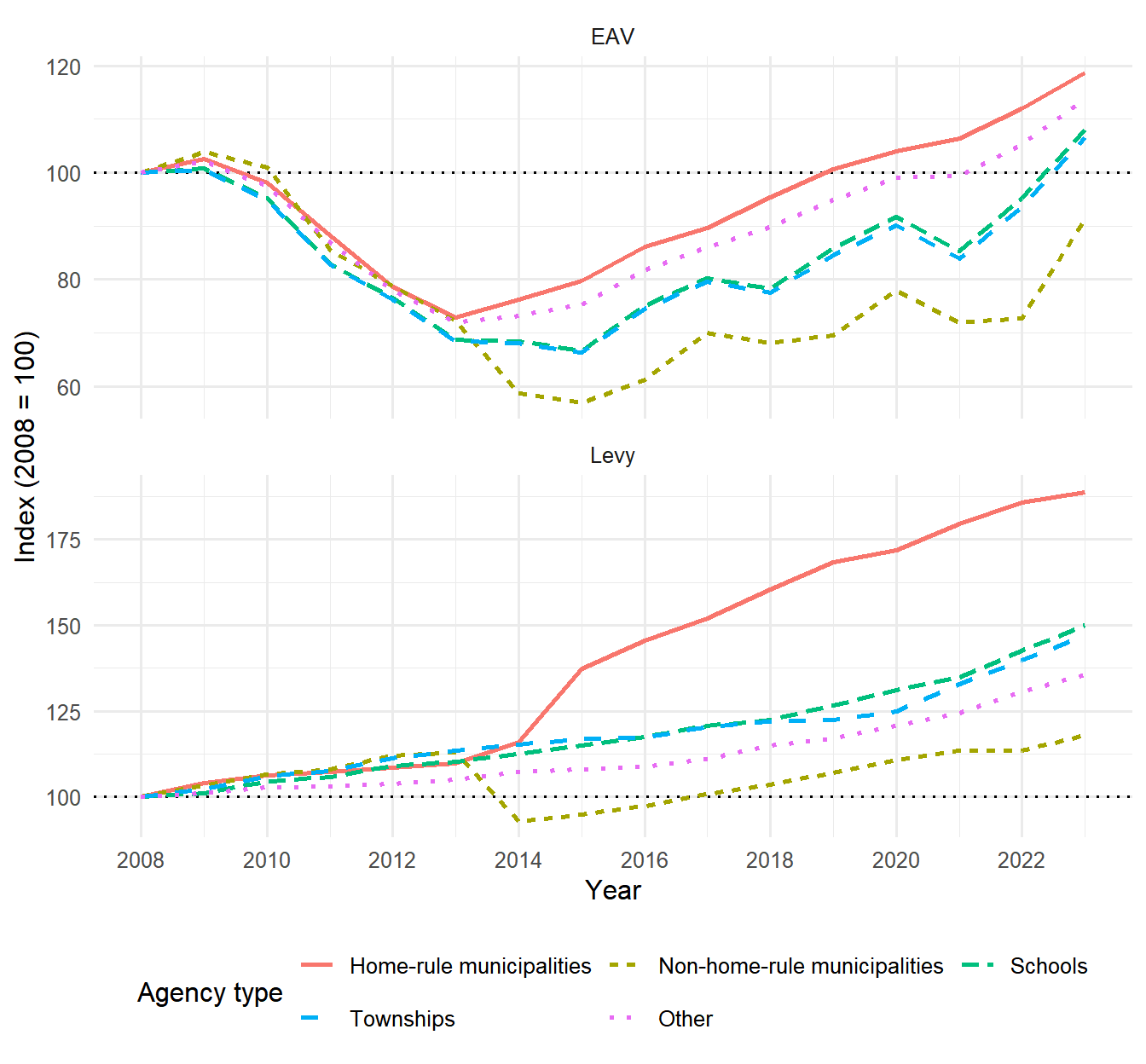
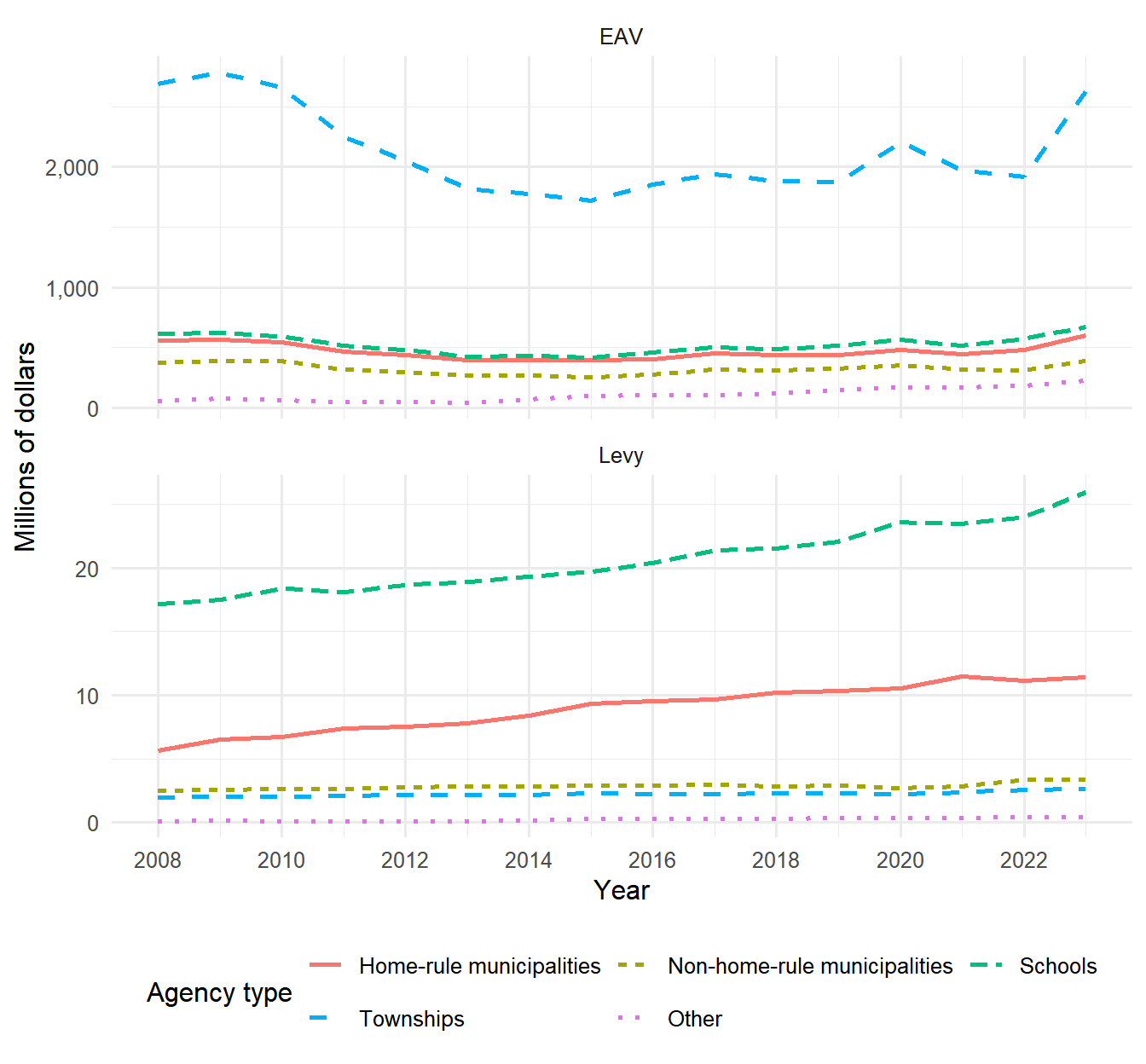
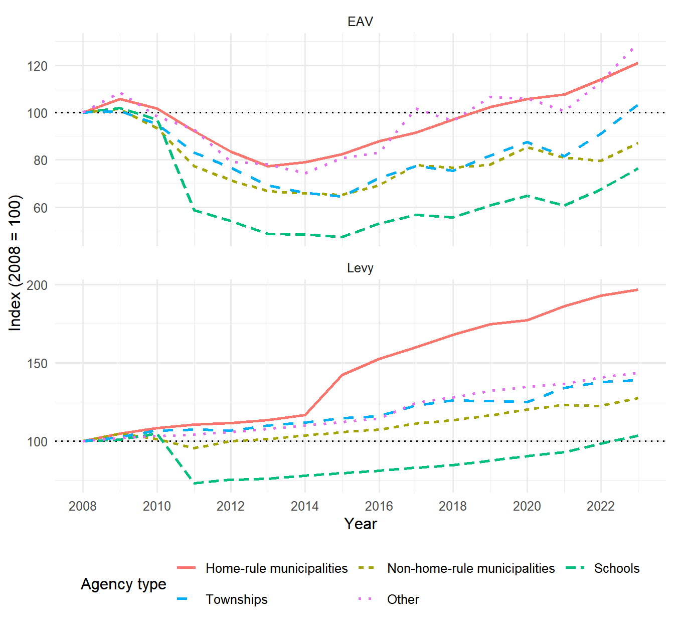
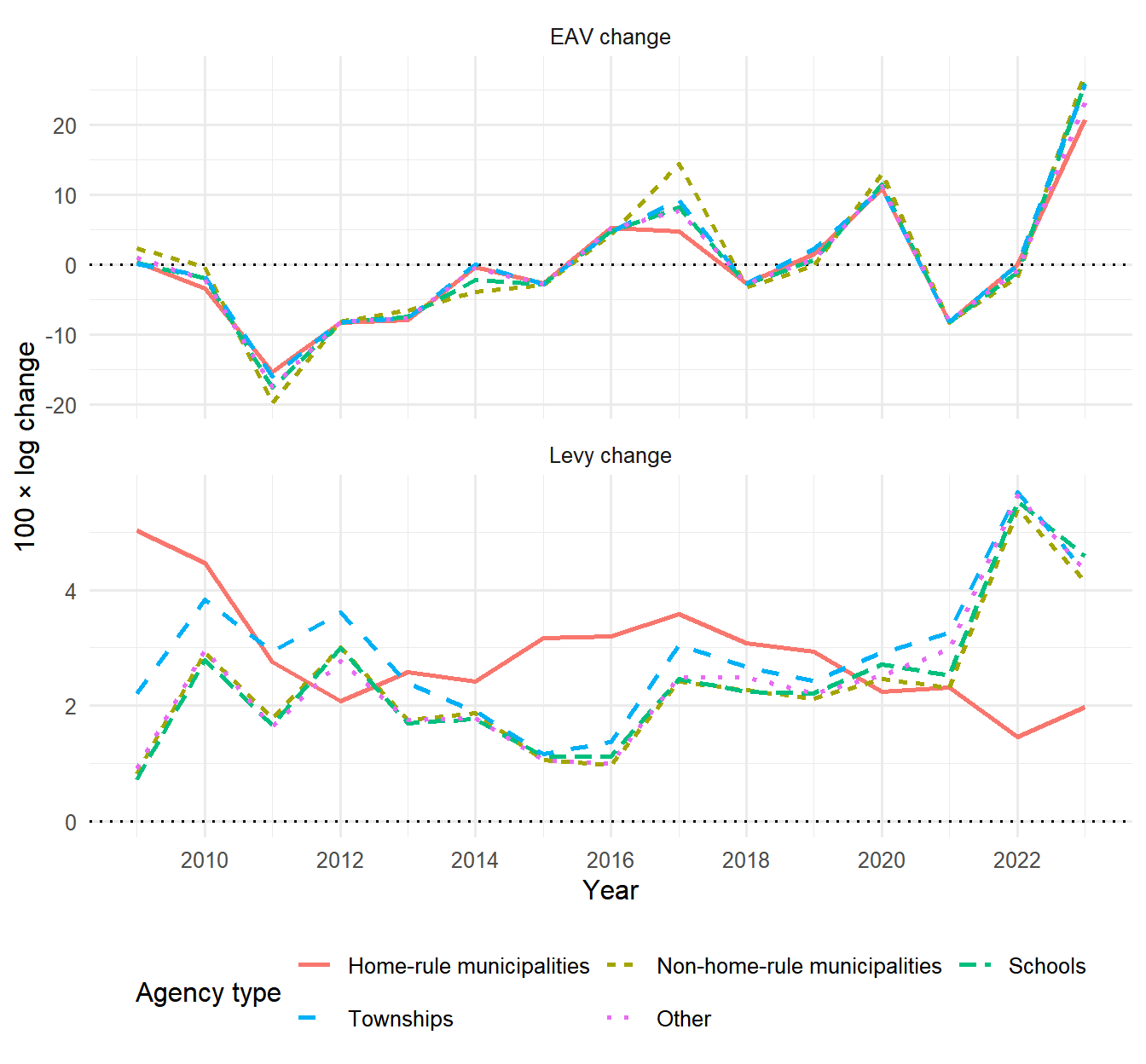
---
title: "Descriptive Statistics and Data Exploration"
subtitle: "Property tax levies and tax bases in Cook County, IL"
format:
html:
toc: true
toc-depth: 3
code-fold: true
code-summary: "Show code"
code-tools: true
df-print: paged
execute:
echo: true
warning: false
message: false
cache: false
---
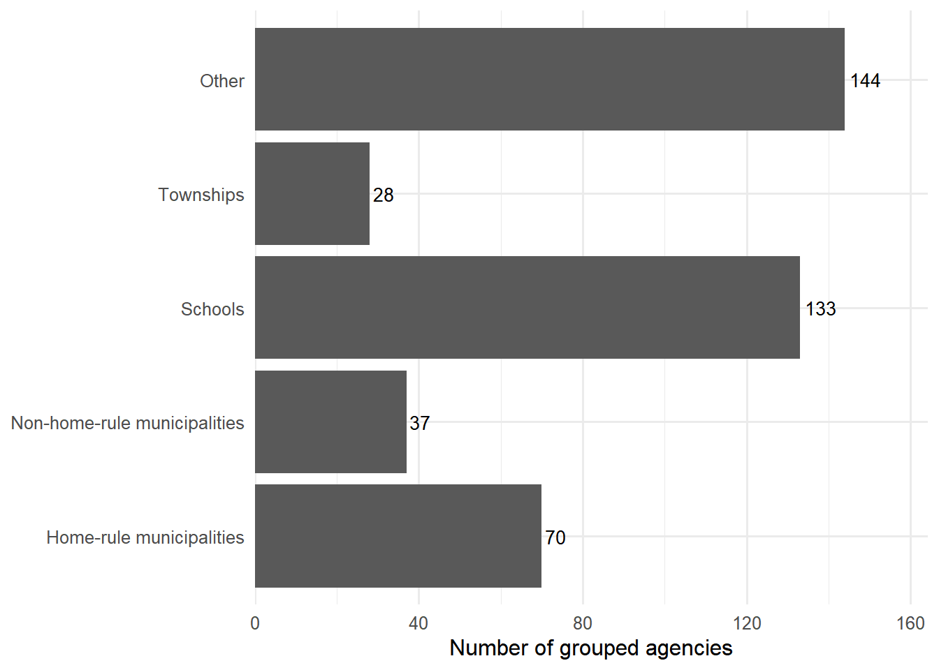
This page compares the source taxing-agency records **before sample exclusions** with the grouped panel used in the corrected manuscript analysis **after exclusions**. Within every comparison, the after-exclusion results appear first and are therefore the default tab.
The annual-change variables follow the corrected model definitions:
- `d_levy` is 100 times the log change in the total final levy.
- `d_eav` is 100 times the log change in equalized assessed value (EAV).
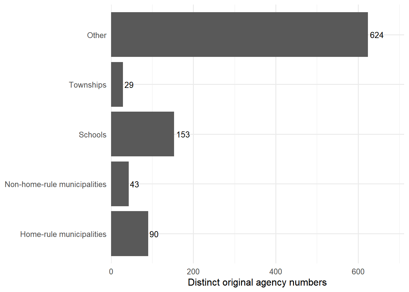
The before-exclusion results use the original PTAXSIM agency number as the unit. The after-exclusion results use the grouped taxing agency used in the manuscript. The two tabs therefore show how both filtering and agency grouping change the sample.
```{r}
#| label: setup
#| echo: false
suppressPackageStartupMessages({
library(tidyverse)
library(haven)
library(scales)
library(knitr)
library(DT)
})
options(scipen = 999)
theme_set(theme_minimal(base_size = 12))
agency_type_levels <- c(
"Home-rule municipalities",
"Non-home-rule municipalities",
"Municipalities (status unavailable)",
"Schools",
"Townships",
"Other"
)
wrap_facet_labels <- function(labels, width = 18) {
stringr::str_wrap(as.character(labels), width = width)
}
agency_facet_labeller <- ggplot2::labeller(
agency_type = function(labels) wrap_facet_labels(labels, width = 18)
)
# -----------------------------
# AFTER EXCLUSIONS: manuscript panel
# -----------------------------
data_file <- "NTA_data_2024_10_14.csv"
if (!file.exists(data_file)) {
stop("Could not find ", data_file, ". Place this QMD in the project root.")
}
main_df <- readr::read_csv(data_file, show_col_types = FALSE)
agency_lookup_file <- "Necessary_Files/fips_all_agency_name.dta"
if (!file.exists(agency_lookup_file)) stop("Could not find ", agency_lookup_file)
agency_lookup <- haven::read_dta(agency_lookup_file) |>
select(agency_group, fipsid) |>
distinct()
main_df <- main_df |>
select(-any_of("fipsid")) |>
left_join(agency_lookup, by = "agency_group") |>
filter(!is.na(fipsid))
census_file <- "Necessary_Files/census_data.dta"
if (!file.exists(census_file)) stop("Could not find ", census_file)
census_df <- haven::read_dta(census_file) |>
select(fipsid, year, any_of(c("total_ig_revenue", "enrollment"))) |>
distinct()
main_df <- main_df |>
select(-any_of(c("total_ig_revenue", "enrollment"))) |>
left_join(census_df, by = c("fipsid", "year"))
if (!"eq_factor_final" %in% names(main_df)) {
if (file.exists("eq_factor.dta")) {
eq_factor <- haven::read_dta("eq_factor.dta")
} else if (file.exists("Necessary_Files/eq_factor.csv")) {
eq_factor <- readr::read_csv(
"Necessary_Files/eq_factor.csv",
show_col_types = FALSE
)
} else {
stop("Could not find eq_factor.dta or Necessary_Files/eq_factor.csv")
}
main_df <- main_df |>
left_join(
eq_factor |> select(year, eq_factor_final) |> distinct(),
by = "year"
)
}
numeric_vars <- c(
"av", "eq_factor_final", "total_final_levy",
"total_ig_revenue", "enrollment", "reassess_year", "home_rule_ind"
)
main_df <- main_df |>
mutate(
across(
any_of(numeric_vars),
~ readr::parse_number(as.character(.x), na = c("NA", "", "."))
)
)
if (!"uniqueid" %in% names(main_df)) {
main_df <- main_df |> mutate(uniqueid = agency_group)
}
required_vars <- c(
"agency_group", "uniqueid", "year", "type", "home_rule_ind",
"reassess_year", "av", "eq_factor_final", "total_final_levy"
)
missing_vars <- setdiff(required_vars, names(main_df))
if (length(missing_vars) > 0) {
stop("Missing required variables: ", paste(missing_vars, collapse = ", "))
}
main_df <- main_df |>
mutate(
n_agency_group = as.integer(factor(agency_group)),
n_uniqueid = as.integer(factor(uniqueid))
) |>
filter(year >= 2008) |>
arrange(n_agency_group, year) |>
group_by(n_agency_group) |>
mutate(
lag_av = lag(av),
lag_eq_factor_final = lag(eq_factor_final),
eav = av * eq_factor_final,
d_eav = 100 * log(
(av * eq_factor_final) /
(lag_av * lag_eq_factor_final)
),
d_levy = 100 * log(total_final_levy / lag(total_final_levy)),
d_total_ig_revenue = 100 * log(
total_ig_revenue / lag(total_ig_revenue)
),
d_enrollment = 100 * log(enrollment / lag(enrollment))
) |>
ungroup() |>
mutate(
type_2 = case_when(
type == "Muni" & home_rule_ind == 1 ~ "HR_muni",
type == "Muni" & home_rule_ind == 0 ~ "NonHR_muni",
TRUE ~ as.character(type)
),
agency_type = case_when(
type_2 == "HR_muni" ~ "Home-rule municipalities",
type_2 == "NonHR_muni" ~ "Non-home-rule municipalities",
type_2 == "School" ~ "Schools",
type_2 == "Township" ~ "Townships",
type_2 == "Other" ~ "Other",
TRUE ~ type_2
),
agency_type = factor(agency_type, levels = agency_type_levels),
agency_id = as.character(n_uniqueid),
agency_name_display = agency_group,
reassessment_status = if_else(
reassess_year == 1,
"Reassessment year",
"Other year"
)
)
first_level_year <- min(main_df$year, na.rm = TRUE)
last_year <- max(main_df$year, na.rm = TRUE)
latest_year <- last_year
analysis_df <- main_df |> filter(year > first_level_year)
first_change_year <- min(analysis_df$year, na.rm = TRUE)
# -----------------------------
# BEFORE EXCLUSIONS: joined PTAXSIM records
# -----------------------------
raw_file_candidates <- c("agency_raw_joined.csv", "raw_agency_joined.csv")
raw_agency_file <- raw_file_candidates[file.exists(raw_file_candidates)][1]
first_existing_numeric <- function(df, candidates) {
nm <- candidates[candidates %in% names(df)][1]
if (length(nm) == 0 || is.na(nm)) return(rep(NA_real_, nrow(df)))
readr::parse_number(as.character(df[[nm]]), na = c("NA", "", "."))
}
first_existing_character <- function(df, candidates, fallback = NA_character_) {
nm <- candidates[candidates %in% names(df)][1]
if (length(nm) == 0 || is.na(nm)) return(rep(fallback, nrow(df)))
as.character(df[[nm]])
}
if (length(raw_agency_file) == 0 || is.na(raw_agency_file)) {
raw_agency_data <- NULL
before_df <- NULL
before_change_df <- NULL
before_available <- FALSE
} else {
raw_agency_data <- readr::read_csv(
raw_agency_file,
col_types = readr::cols(
agency_num = readr::col_character(),
year = readr::col_double(),
.default = readr::col_guess()
),
show_col_types = FALSE
)
raw_id <- first_existing_character(
raw_agency_data,
c("agency_num", "uniqueid", "agency_group")
)
raw_name <- first_existing_character(
raw_agency_data,
c("agency_name", "agency_group", "clean_name")
)
raw_minor_type <- first_existing_character(
raw_agency_data,
c("minor_type", "agency_minor_type")
)
raw_major_type <- first_existing_character(
raw_agency_data,
c("major_type", "agency_major_type")
)
raw_home_rule <- first_existing_numeric(raw_agency_data, "home_rule_ind")
raw_reassess <- first_existing_numeric(raw_agency_data, "reassess_year")
raw_levy <- first_existing_numeric(raw_agency_data, "total_final_levy")
raw_rate <- first_existing_numeric(raw_agency_data, "total_final_rate")
raw_eav <- first_existing_numeric(
raw_agency_data,
c("cty_total_eav", "eav", "total_eav")
)
# Match the earlier cleaning logic only to recover missing EAV values. No
# records are excluded here. Invalid or nonpositive values remain in the
# source data but cannot be used in logarithmic changes.
raw_eav <- if_else(
is.na(raw_eav) & raw_levy > 0 & raw_rate > 0,
raw_levy / (raw_rate / 100),
raw_eav
)
raw_year <- first_existing_numeric(raw_agency_data, "year")
before_df <- raw_agency_data |>
mutate(
agency_id = raw_id,
agency_name_display = if_else(
is.na(raw_name) | raw_name == "",
raw_id,
raw_name
),
year = as.integer(raw_year),
original_minor_type = raw_minor_type,
original_major_type = raw_major_type,
home_rule_ind = raw_home_rule,
reassess_year = raw_reassess,
total_final_levy = raw_levy,
eav = raw_eav,
agency_type = case_when(
original_minor_type == "MUNI" & home_rule_ind == 1 ~
"Home-rule municipalities",
original_minor_type == "MUNI" & home_rule_ind == 0 ~
"Non-home-rule municipalities",
original_minor_type == "MUNI" ~
"Municipalities (status unavailable)",
original_minor_type %in% c("ELEMENTARY", "SECONDARY", "UNIFIED") ~
"Schools",
original_minor_type == "TOWNSHIP" ~ "Townships",
TRUE ~ "Other"
),
agency_type = factor(agency_type, levels = agency_type_levels),
reassessment_status = if_else(
reassess_year == 1,
"Reassessment year",
"Other year"
)
) |>
filter(
!is.na(agency_id),
!is.na(year),
year >= first_level_year,
year <= last_year
) |>
distinct(agency_id, year, .keep_all = TRUE) |>
arrange(agency_id, year) |>
group_by(agency_id) |>
mutate(
d_levy = 100 * log(total_final_levy / lag(total_final_levy)),
d_eav = 100 * log(eav / lag(eav))
) |>
ungroup()
before_change_df <- before_df |> filter(year > first_level_year)
before_available <- nrow(before_df) > 0
}
before_missing_message <- paste0(
"The before-exclusion source file was not found. Add agency_raw_joined.csv ",
"or raw_agency_joined.csv to the project root to display this tab."
)
make_overview <- function(df, change_df, id_var, panel_label) {
years <- sort(unique(df$year))
panel_year_count <- length(years)
id_sym <- rlang::ensym(id_var)
years_per_agency <- df |>
distinct(!!id_sym, year) |>
count(!!id_sym, name = "years_observed")
tibble(
Measure = c(
"Panel definition",
"First year",
"Last year",
"Years in panel",
"Agency-year observations",
"Unique taxing-agency units",
"Units observed in every panel year",
"Agency-year observations with a prior year",
"Observations with finite d_levy and d_eav"
),
Value = c(
panel_label,
min(years),
max(years),
panel_year_count,
nrow(df),
n_distinct(df[[rlang::as_name(id_sym)]]),
sum(years_per_agency$years_observed == panel_year_count),
nrow(change_df),
sum(is.finite(change_df$d_levy) & is.finite(change_df$d_eav))
)
)
}
make_long_run_growth <- function(df, id_var) {
id_sym <- rlang::ensym(id_var)
start_values <- df |>
filter(year == first_level_year) |>
transmute(
agency_id = as.character(!!id_sym),
agency_name_display,
agency_type,
start_levy = total_final_levy,
start_eav = eav
)
end_values <- df |>
filter(year == last_year) |>
transmute(
agency_id = as.character(!!id_sym),
end_levy = total_final_levy,
end_eav = eav
)
start_values |>
inner_join(end_values, by = "agency_id") |>
mutate(
levy_growth = 100 * (end_levy - start_levy) / start_levy,
eav_growth = 100 * (end_eav - start_eav) / start_eav,
levy_minus_eav_growth = levy_growth - eav_growth
) |>
filter(
is.finite(levy_growth),
is.finite(eav_growth)
)
}
long_run_growth_after <- make_long_run_growth(main_df, agency_id)
long_run_growth_before <- if (before_available) {
make_long_run_growth(before_df, agency_id)
} else {
NULL
}
```
# Sample composition
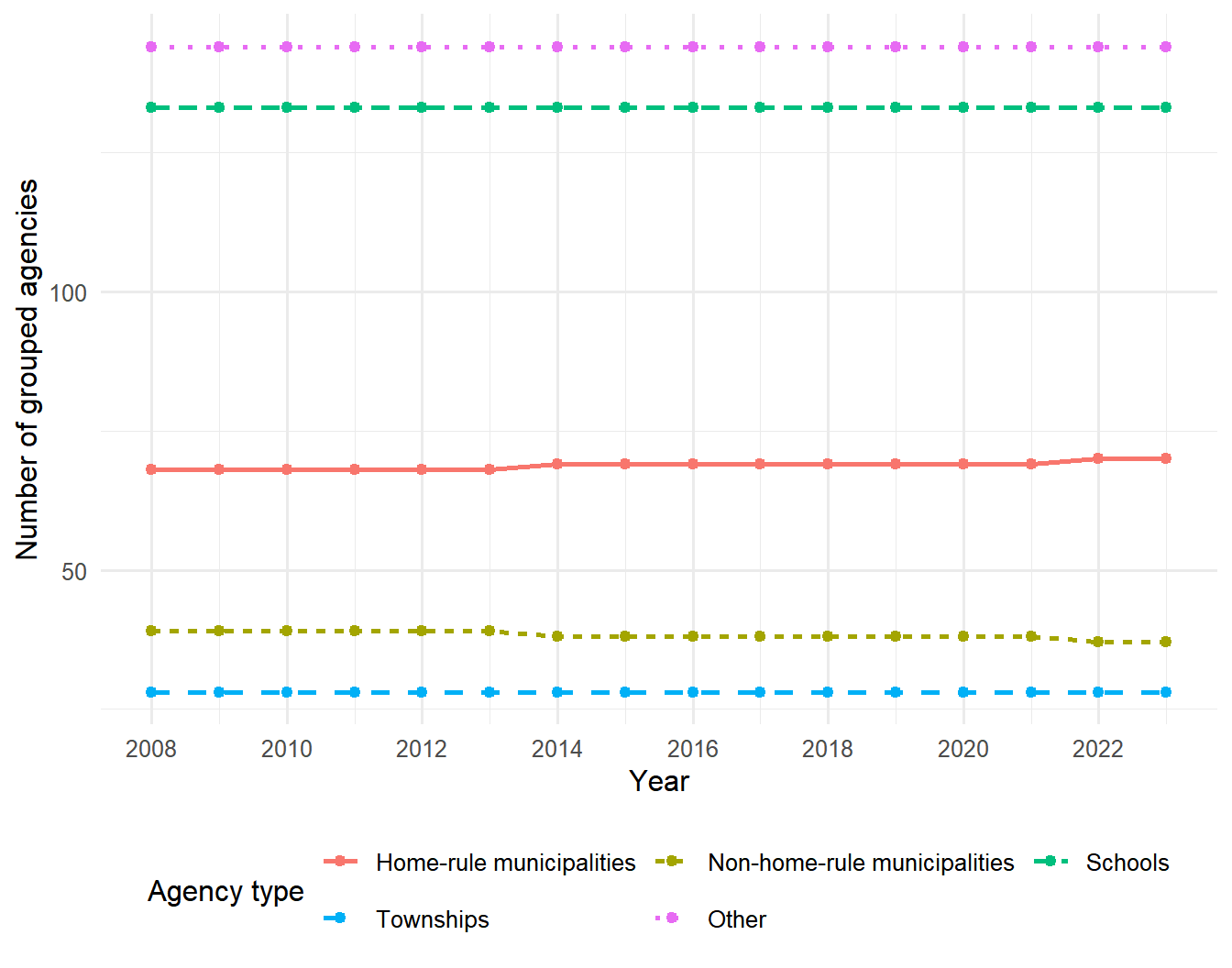
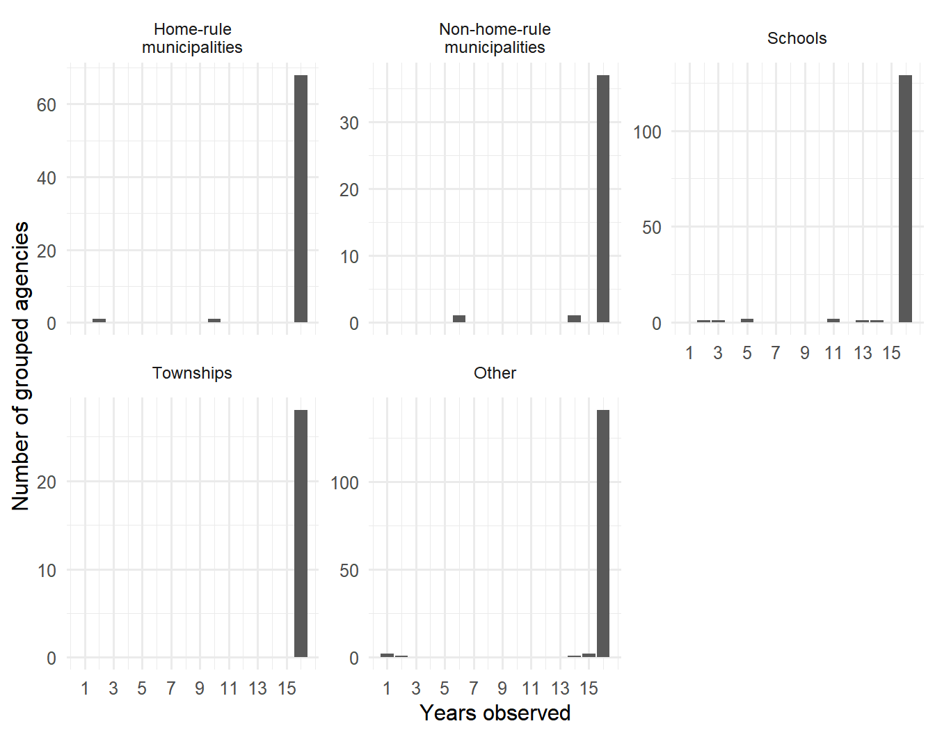
The tabs compare the same `r first_level_year`–`r last_year` period. The before-exclusion tab counts original PTAXSIM agency numbers; the after-exclusion tab counts grouped manuscript agencies.
::: {.panel-tabset}
## After exclusions
### Sample overview
```{r}
#| label: tbl-sample-overview-after
#| tbl-cap: "Overview of the grouped manuscript panel"
sample_overview_after <- make_overview(
  main_df,
  analysis_df,
  agency_id,
  "Grouped taxing agencies after sample exclusions"
)

knitr::kable(sample_overview_after, align = c("l", "r"))
```
### Agencies by type
```{r}
#| label: tbl-agency-counts-after
#| tbl-cap: "Grouped taxing agencies represented in the latest panel year"
agency_counts_after <- main_df |>
  filter(year == latest_year) |>
  distinct(agency_id, agency_type) |>
  count(agency_type, name = "Agencies") |>
  mutate(Share = scales::percent(Agencies / sum(Agencies), accuracy = 0.1))

knitr::kable(
  agency_counts_after,
  col.names = c("Agency type", "Agencies", "Share"),
  align = c("l", "r", "r")
)
```
```{r}
#| label: fig-agency-counts-after
#| fig-cap: "Grouped taxing agencies after sample exclusions"
#| fig-height: 5
agency_counts_after |>
  ggplot(aes(x = agency_type, y = Agencies)) +
  geom_col() +
  geom_text(aes(label = Agencies), hjust = -0.15, size = 3.5) +
  coord_flip() +
  scale_y_continuous(
    labels = scales::comma,
    expand = expansion(mult = c(0, 0.14))
  ) +
  labs(x = NULL, y = "Number of grouped agencies")
```
### Agency counts over time
```{r}
#| label: fig-agency-counts-time-after
#| fig-cap: "Grouped taxing agencies represented in the panel each year"
#| fig-height: 5.5
agency_counts_time_after <- main_df |>
  distinct(year, agency_id, agency_type) |>
  count(year, agency_type, name = "Agencies")

agency_counts_time_after |>
  ggplot(aes(
    x = year,
    y = Agencies,
    group = agency_type,
    color = agency_type,
    linetype = agency_type
  )) +
  geom_line(linewidth = 0.9) +
  geom_point(size = 1.8) +
  scale_x_continuous(breaks = scales::breaks_pretty(n = 8)) +
  labs(
    x = "Year",
    y = "Number of grouped agencies",
    color = "Agency type",
    linetype = "Agency type"
  ) +
  guides(
    color = guide_legend(nrow = 2, byrow = TRUE),
    linetype = guide_legend(nrow = 2, byrow = TRUE)
  ) +
  theme(legend.position = "bottom")
```
### Panel completeness
```{r}
#| label: fig-panel-completeness-after
#| fig-cap: "Years observed for each grouped taxing agency"
#| fig-height: 5.5
panel_completeness_after <- main_df |>
  distinct(agency_id, agency_type, year) |>
  count(agency_id, agency_type, name = "Years observed")

panel_completeness_after |>
  ggplot(aes(x = `Years observed`)) +
  geom_bar() +
  facet_wrap(
    ~agency_type,
    scales = "free_y",
    labeller = agency_facet_labeller
  ) +
  scale_x_continuous(breaks = seq(1, n_distinct(main_df$year), by = 2)) +
  labs(x = "Years observed", y = "Number of grouped agencies") +
  theme(strip.text = element_text(size = 9))
```
```{r}
#| label: tbl-panel-completeness-after
#| tbl-cap: "Panel completeness after exclusions"
panel_completeness_after |>
  group_by(agency_type) |>
  summarise(
    Agencies = n(),
    `Minimum years` = min(`Years observed`),
    `Median years` = median(`Years observed`),
    `Maximum years` = max(`Years observed`),
    `Observed every year` = sum(`Years observed` == n_distinct(main_df$year)),
    .groups = "drop"
  ) |>
  knitr::kable(align = c("l", rep("r", 5)))
```
## Before exclusions
The source data tab retains all original agency types and does not apply the Cook County share, home-rule-status, agency-type, levy, or grouped-agency exclusions. Calculations that require positive, nonmissing levy or EAV values necessarily use only records on which those quantities can be calculated.
```{r}
#| label: tbl-sample-overview-before
#| tbl-cap: "Overview of the joined PTAXSIM source records"
if (!before_available) {
  cat(before_missing_message)
} else {
  make_overview(
    before_df,
    before_change_df,
    agency_id,
    "Original PTAXSIM agency numbers before sample exclusions"
  ) |>
    knitr::kable(align = c("l", "r"))
}
```
### Agencies by manuscript category
```{r}
#| label: tbl-agency-counts-before
#| tbl-cap: "Original agency numbers represented in the latest comparison year"
if (!before_available) {
  cat(before_missing_message)
} else {
  agency_counts_before <- before_df |>
    filter(year == latest_year) |>
    distinct(agency_id, agency_type) |>
    count(agency_type, name = "Agencies") |>
    mutate(Share = scales::percent(Agencies / sum(Agencies), accuracy = 0.1))

  knitr::kable(
    agency_counts_before,
    col.names = c("Agency type", "Agency numbers", "Share"),
    align = c("l", "r", "r")
  )
}
```
```{r}
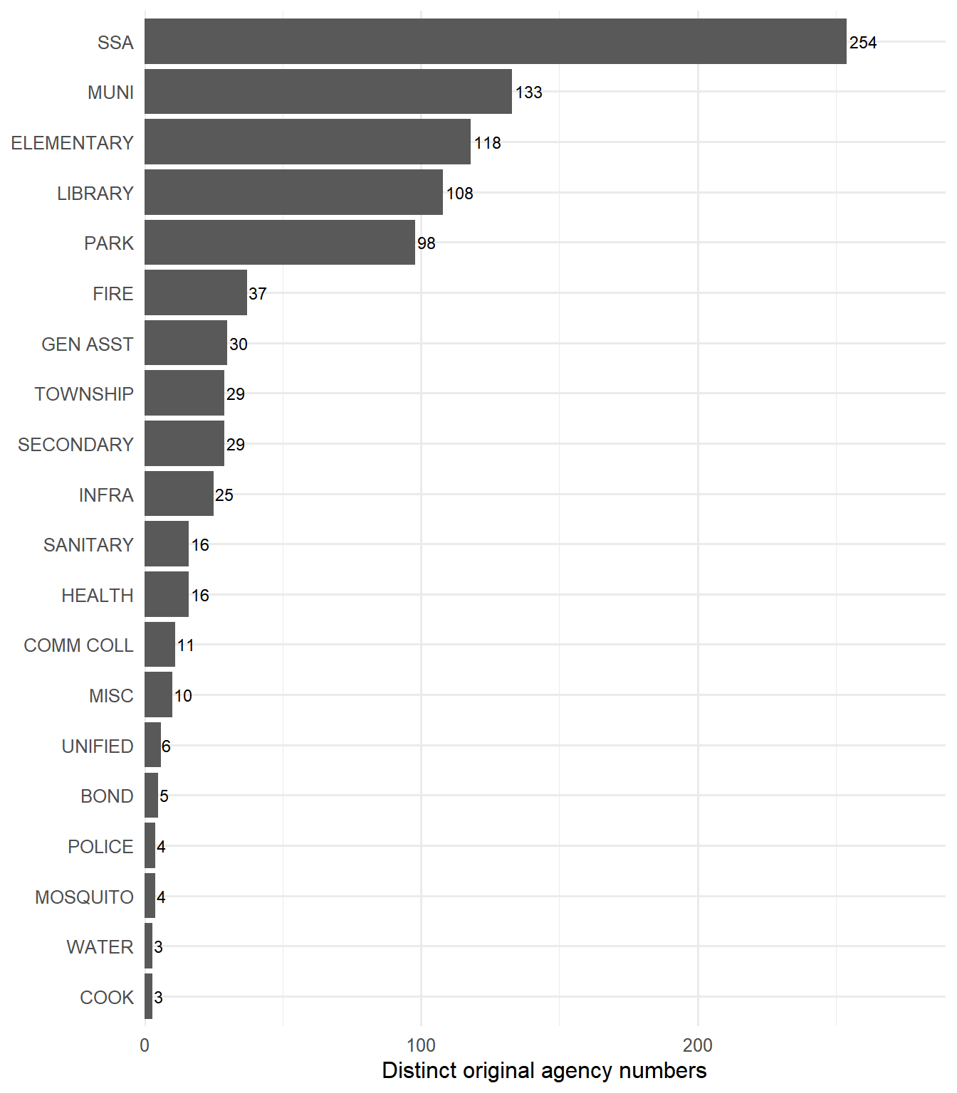
#| label: fig-agency-counts-before
#| fig-cap: "Original agency numbers before sample exclusions"
#| fig-height: 5
if (!before_available) {
  cat(before_missing_message)
} else {
  agency_counts_before |>
    ggplot(aes(x = agency_type, y = Agencies)) +
    geom_col() +
    geom_text(aes(label = Agencies), hjust = -0.15, size = 3.5) +
    coord_flip() +
    scale_y_continuous(
      labels = scales::comma,
      expand = expansion(mult = c(0, 0.14))
    ) +
    labs(x = NULL, y = "Distinct original agency numbers")
}
```
### Original PTAXSIM minor types
```{r}
#| label: fig-original-minor-types-before
#| fig-cap: "Original PTAXSIM agency types before sample exclusions"
#| fig-height: 8
if (!before_available) {
  cat(before_missing_message)
} else {
  before_df |>
    filter(year == latest_year, !is.na(original_minor_type)) |>
    distinct(agency_id, original_minor_type) |>
    count(original_minor_type, name = "Agencies", sort = TRUE) |>
    ggplot(aes(x = reorder(original_minor_type, Agencies), y = Agencies)) +
    geom_col() +
    geom_text(aes(label = scales::comma(Agencies)), hjust = -0.1, size = 3) +
    coord_flip() +
    scale_y_continuous(
      labels = scales::comma,
      expand = expansion(mult = c(0, 0.14))
    ) +
    labs(x = NULL, y = "Distinct original agency numbers")
}
```
### Agency counts over time
```{r}
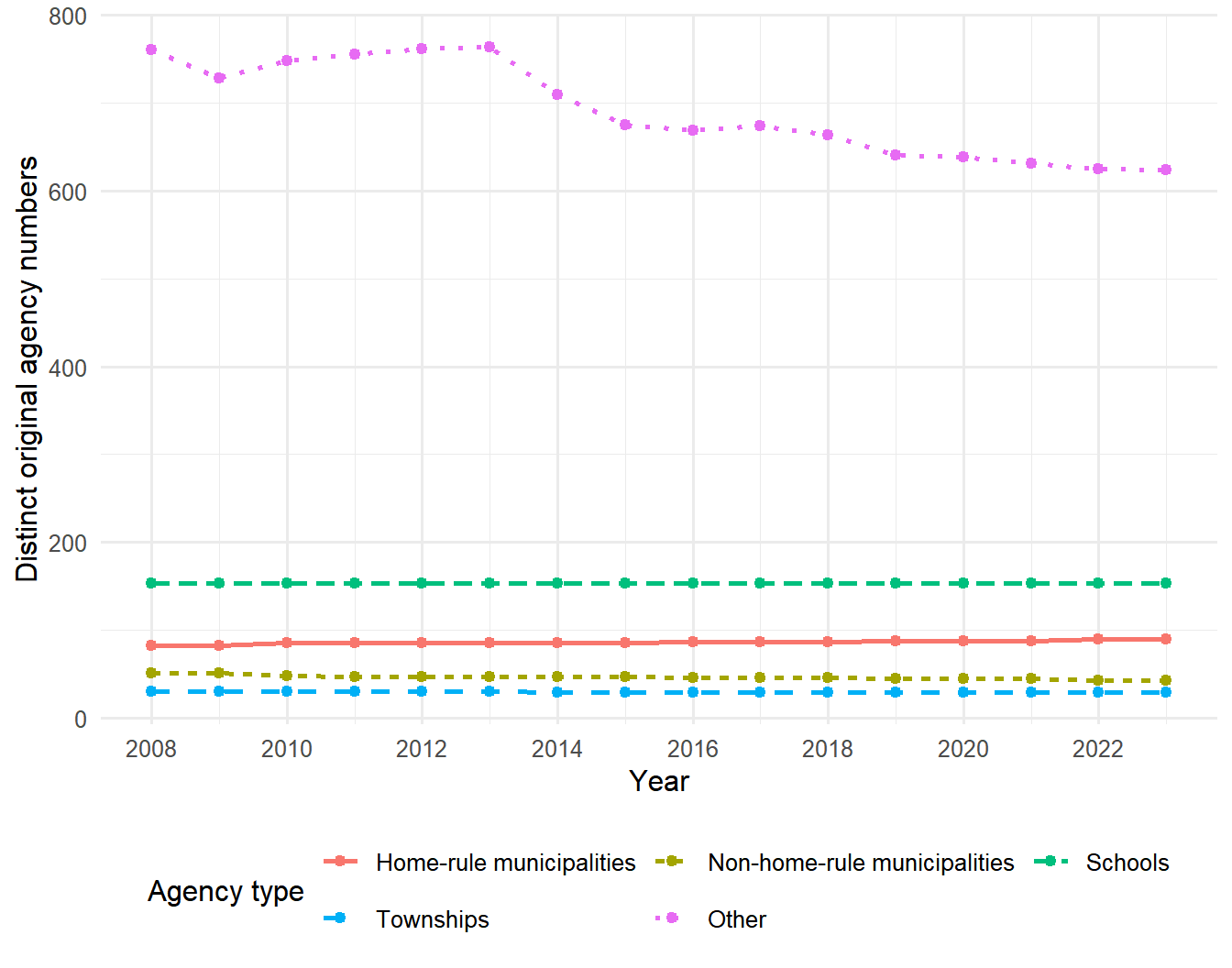
#| label: fig-agency-counts-time-before
#| fig-cap: "Original agency numbers represented in the source data each year"
#| fig-height: 5.5
if (!before_available) {
  cat(before_missing_message)
} else {
  agency_counts_time_before <- before_df |>
    distinct(year, agency_id, agency_type) |>
    count(year, agency_type, name = "Agencies")

  agency_counts_time_before |>
    ggplot(aes(
      x = year,
      y = Agencies,
      group = agency_type,
      color = agency_type,
      linetype = agency_type
    )) +
    geom_line(linewidth = 0.9) +
    geom_point(size = 1.8) +
    scale_x_continuous(breaks = scales::breaks_pretty(n = 8)) +
    labs(
      x = "Year",
      y = "Distinct original agency numbers",
      color = "Agency type",
      linetype = "Agency type"
    ) +
    guides(
      color = guide_legend(nrow = 2, byrow = TRUE),
      linetype = guide_legend(nrow = 2, byrow = TRUE)
    ) +
    theme(legend.position = "bottom")
}
```
### Panel completeness
```{r}
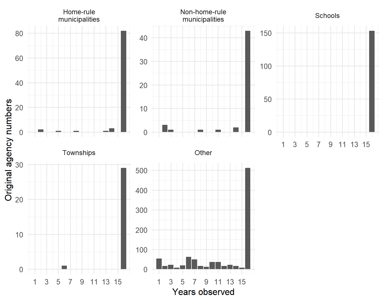
#| label: fig-panel-completeness-before
#| fig-cap: "Years observed for each original agency number"
#| fig-height: 5.5
if (!before_available) {
  cat(before_missing_message)
} else {
  panel_completeness_before <- before_df |>
    distinct(agency_id, agency_type, year) |>
    count(agency_id, agency_type, name = "Years observed")

  panel_completeness_before |>
    ggplot(aes(x = `Years observed`)) +
    geom_bar() +
    facet_wrap(
      ~agency_type,
      scales = "free_y",
      labeller = agency_facet_labeller
    ) +
    scale_x_continuous(breaks = seq(1, n_distinct(before_df$year), by = 2)) +
    labs(x = "Years observed", y = "Original agency numbers") +
    theme(strip.text = element_text(size = 9))
}
```
```{r}
#| label: tbl-panel-completeness-before
#| tbl-cap: "Panel completeness before exclusions"
if (!before_available) {
  cat(before_missing_message)
} else {
  panel_completeness_before |>
    group_by(agency_type) |>
    summarise(
      Agencies = n(),
      `Minimum years` = min(`Years observed`),
      `Median years` = median(`Years observed`),
      `Maximum years` = max(`Years observed`),
      `Observed every year` = sum(`Years observed` == n_distinct(before_df$year)),
      .groups = "drop"
    ) |>
    knitr::kable(align = c("l", rep("r", 5)))
}
```
### Searchable source-agency inventory
```{r}
#| label: tbl-raw-agency-inventory
if (!before_available) {
  cat(before_missing_message)
} else {
  raw_agency_inventory <- before_df |>
    group_by(
      agency_id,
      agency_name_display,
      original_major_type,
      original_minor_type
    ) |>
    summarise(
      `First year` = min(year, na.rm = TRUE),
      `Last year` = max(year, na.rm = TRUE),
      `Years observed` = n_distinct(year),
      .groups = "drop"
    ) |>
    arrange(agency_name_display) |>
    rename(
      `Agency number` = agency_id,
      `Agency name` = agency_name_display,
      `Major type` = original_major_type,
      `Minor type` = original_minor_type
    )

  DT::datatable(
    raw_agency_inventory,
    rownames = FALSE,
    filter = "top",
    class = "compact stripe hover",
    options = list(
      pageLength = 15,
      lengthMenu = list(
        c(10, 15, 25, 50, 100, -1),
        c("10", "15", "25", "50", "100", "All")
      ),
      order = list(list(1, "asc")),
      scrollX = TRUE,
      autoWidth = TRUE
    )
  )
}
```
:::
# Levy and tax-base levels
::: {.panel-tabset}
## After exclusions
### Latest-year snapshot
```{r}
#| label: tbl-latest-levels-after
#| tbl-cap: "Levy and EAV levels after exclusions"
latest_levels_after <- main_df |>
  filter(year == latest_year) |>
  group_by(agency_type) |>
  summarise(
    Agencies = n_distinct(agency_id),
    `Median levy ($ millions)` = median(total_final_levy, na.rm = TRUE) / 1e6,
    `Total levy ($ billions)` = sum(total_final_levy, na.rm = TRUE) / 1e9,
    `Median EAV ($ millions)` = median(eav, na.rm = TRUE) / 1e6,
    `Total EAV ($ billions)` = sum(eav, na.rm = TRUE) / 1e9,
    .groups = "drop"
  ) |>
  mutate(across(where(is.numeric), ~ round(.x, 2)))

knitr::kable(latest_levels_after, align = c("l", rep("r", 5)))
```
### Median levels over time
```{r}
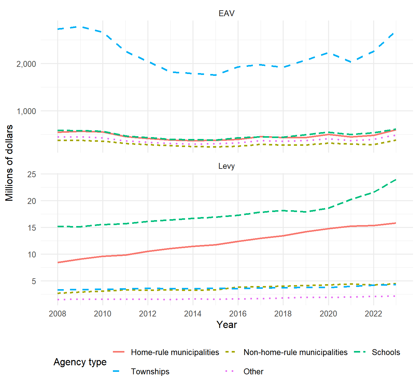
#| label: fig-median-levels-after
#| fig-cap: "Median levy and EAV after exclusions"
#| fig-height: 6.5
median_levels_after <- main_df |>
  select(year, agency_type, Levy = total_final_levy, EAV = eav) |>
  pivot_longer(c(Levy, EAV), names_to = "Measure", values_to = "Value") |>
  group_by(year, agency_type, Measure) |>
  summarise(`Median value` = median(Value, na.rm = TRUE) / 1e6, .groups = "drop")

median_levels_after |>
  ggplot(aes(
    x = year,
    y = `Median value`,
    group = agency_type,
    color = agency_type,
    linetype = agency_type
  )) +
  geom_line(linewidth = 0.9) +
  facet_wrap(~Measure, scales = "free_y", ncol = 1) +
  scale_x_continuous(breaks = scales::breaks_pretty(n = 8)) +
  scale_y_continuous(labels = scales::label_comma()) +
  labs(
    x = "Year",
    y = "Millions of dollars",
    color = "Agency type",
    linetype = "Agency type"
  ) +
  guides(
    color = guide_legend(nrow = 2, byrow = TRUE),
    linetype = guide_legend(nrow = 2, byrow = TRUE)
  ) +
  theme(legend.position = "bottom")
```
### Indexed aggregate growth
```{r}
#| label: fig-indexed-levels-after
#| fig-cap: "Aggregate levy and EAV after exclusions, indexed to the first panel year"
#| fig-height: 6.5
indexed_levels_after <- main_df |>
  select(year, agency_type, Levy = total_final_levy, EAV = eav) |>
  pivot_longer(c(Levy, EAV), names_to = "Measure", values_to = "Value") |>
  group_by(year, agency_type, Measure) |>
  summarise(Total = sum(Value, na.rm = TRUE), .groups = "drop") |>
  group_by(agency_type, Measure) |>
  arrange(year, .by_group = TRUE) |>
  mutate(Index = 100 * Total / first(Total)) |>
  ungroup()

indexed_levels_after |>
  ggplot(aes(
    x = year,
    y = Index,
    group = agency_type,
    color = agency_type,
    linetype = agency_type
  )) +
  geom_hline(yintercept = 100, linetype = "dotted") +
  geom_line(linewidth = 0.9) +
  facet_wrap(~Measure, ncol = 1, scales = "free_y") +
  scale_x_continuous(breaks = scales::breaks_pretty(n = 8)) +
  labs(
    x = "Year",
    y = paste0("Index (", first_level_year, " = 100)"),
    color = "Agency type",
    linetype = "Agency type"
  ) +
  guides(
    color = guide_legend(nrow = 2, byrow = TRUE),
    linetype = guide_legend(nrow = 2, byrow = TRUE)
  ) +
  theme(legend.position = "bottom")
```
## Before exclusions
### Latest-year snapshot
```{r}
#| label: tbl-latest-levels-before
#| tbl-cap: "Levy and EAV levels before exclusions"
if (!before_available) {
  cat(before_missing_message)
} else {
  before_df |>
    filter(year == latest_year) |>
    group_by(agency_type) |>
    summarise(
      Agencies = n_distinct(agency_id),
      `Valid levy values` = sum(is.finite(total_final_levy)),
      `Median levy ($ millions)` = median(total_final_levy, na.rm = TRUE) / 1e6,
      `Total levy ($ billions)` = sum(total_final_levy, na.rm = TRUE) / 1e9,
      `Valid EAV values` = sum(is.finite(eav)),
      `Median EAV ($ millions)` = median(eav, na.rm = TRUE) / 1e6,
      `Total EAV ($ billions)` = sum(eav, na.rm = TRUE) / 1e9,
      .groups = "drop"
    ) |>
    mutate(across(where(is.numeric), ~ round(.x, 2))) |>
    knitr::kable(align = c("l", rep("r", 7)))
}
```
### Median levels over time
```{r}
#| label: fig-median-levels-before
#| fig-cap: "Median levy and EAV before exclusions"
#| fig-height: 6.5
if (!before_available) {
  cat(before_missing_message)
} else {
  median_levels_before <- before_df |>
    select(year, agency_type, Levy = total_final_levy, EAV = eav) |>
    pivot_longer(c(Levy, EAV), names_to = "Measure", values_to = "Value") |>
    filter(is.finite(Value)) |>
    group_by(year, agency_type, Measure) |>
    summarise(`Median value` = median(Value, na.rm = TRUE) / 1e6, .groups = "drop")

  median_levels_before |>
    ggplot(aes(
      x = year,
      y = `Median value`,
      group = agency_type,
      color = agency_type,
      linetype = agency_type
    )) +
    geom_line(linewidth = 0.9) +
    facet_wrap(~Measure, scales = "free_y", ncol = 1) +
    scale_x_continuous(breaks = scales::breaks_pretty(n = 8)) +
    scale_y_continuous(labels = scales::label_comma()) +
    labs(
      x = "Year",
      y = "Millions of dollars",
      color = "Agency type",
      linetype = "Agency type"
    ) +
    guides(
      color = guide_legend(nrow = 2, byrow = TRUE),
      linetype = guide_legend(nrow = 2, byrow = TRUE)
    ) +
    theme(legend.position = "bottom")
}
```
### Indexed aggregate growth
```{r}
#| label: fig-indexed-levels-before
#| fig-cap: "Aggregate levy and EAV before exclusions, indexed to the first panel year"
#| fig-height: 6.5
if (!before_available) {
  cat(before_missing_message)
} else {
  indexed_levels_before <- before_df |>
    select(year, agency_type, Levy = total_final_levy, EAV = eav) |>
    pivot_longer(c(Levy, EAV), names_to = "Measure", values_to = "Value") |>
    filter(is.finite(Value)) |>
    group_by(year, agency_type, Measure) |>
    summarise(Total = sum(Value, na.rm = TRUE), .groups = "drop") |>
    group_by(agency_type, Measure) |>
    arrange(year, .by_group = TRUE) |>
    filter(first(Total) > 0) |>
    mutate(Index = 100 * Total / first(Total)) |>
    ungroup()

  indexed_levels_before |>
    ggplot(aes(
      x = year,
      y = Index,
      group = agency_type,
      color = agency_type,
      linetype = agency_type
    )) +
    geom_hline(yintercept = 100, linetype = "dotted") +
    geom_line(linewidth = 0.9) +
    facet_wrap(~Measure, ncol = 1, scales = "free_y") +
    scale_x_continuous(breaks = scales::breaks_pretty(n = 8)) +
    labs(
      x = "Year",
      y = paste0("Index (", first_level_year, " = 100)"),
      color = "Agency type",
      linetype = "Agency type"
    ) +
    guides(
      color = guide_legend(nrow = 2, byrow = TRUE),
      linetype = guide_legend(nrow = 2, byrow = TRUE)
    ) +
    theme(legend.position = "bottom")
}
```
:::
# Annual changes
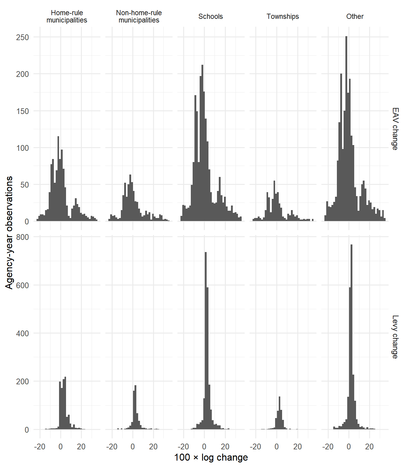
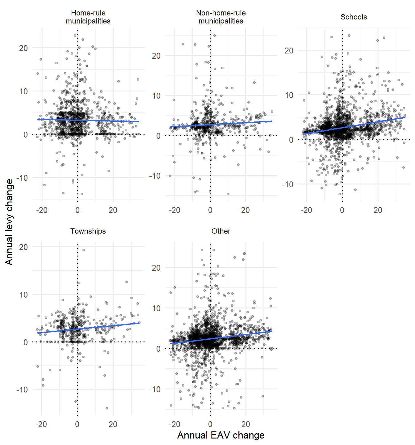
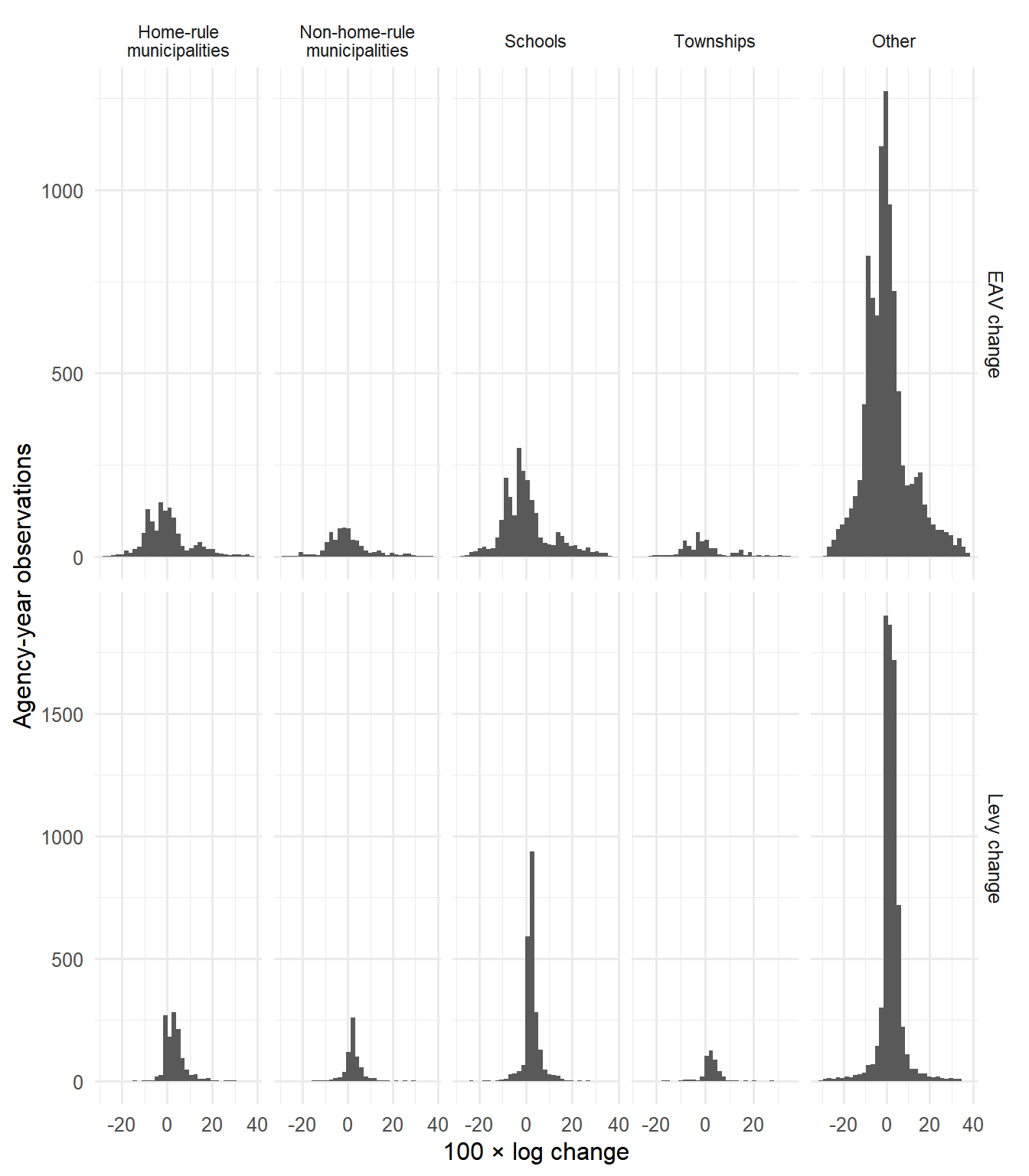
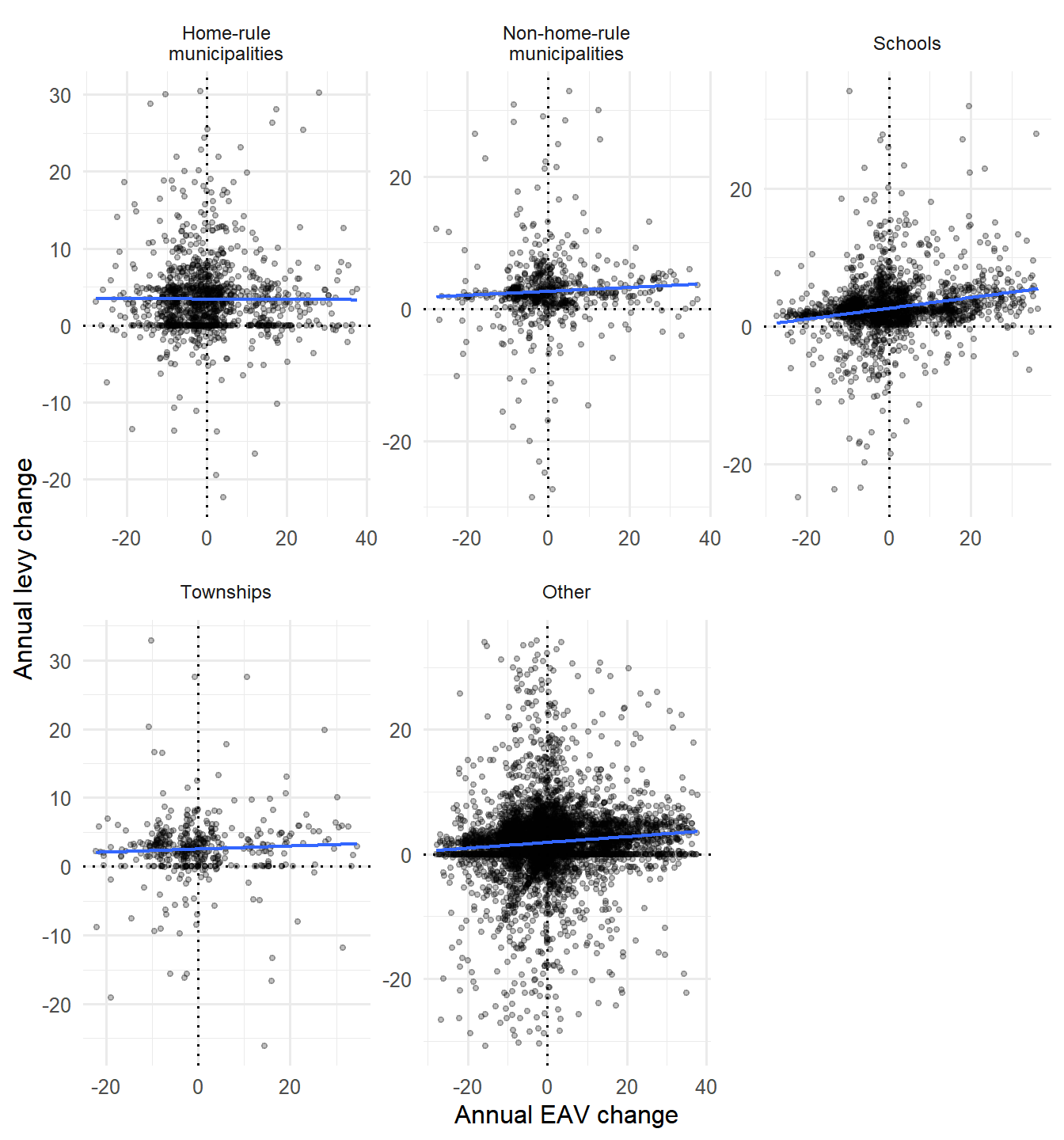
The distribution and scatter plots trim the first and ninety-ninth percentiles **for display only**. The summary statistics retain all finite annual changes.
::: {.panel-tabset}
## After exclusions
### Summary statistics
```{r}
#| label: tbl-change-summary-after
#| tbl-cap: "Annual levy and EAV changes after exclusions"
change_summary_after <- analysis_df |>
  group_by(agency_type) |>
  summarise(
    N = sum(is.finite(d_levy) & is.finite(d_eav)),
    `Mean d_levy` = mean(d_levy[is.finite(d_levy)], na.rm = TRUE),
    `Median d_levy` = median(d_levy[is.finite(d_levy)], na.rm = TRUE),
    `SD d_levy` = sd(d_levy[is.finite(d_levy)], na.rm = TRUE),
    `Mean d_eav` = mean(d_eav[is.finite(d_eav)], na.rm = TRUE),
    `Median d_eav` = median(d_eav[is.finite(d_eav)], na.rm = TRUE),
    `SD d_eav` = sd(d_eav[is.finite(d_eav)], na.rm = TRUE),
    .groups = "drop"
  ) |>
  mutate(across(where(is.numeric), ~ round(.x, 2)))

knitr::kable(change_summary_after, align = c("l", rep("r", 7)))
```
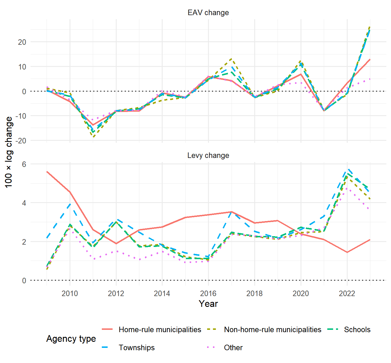
### Median annual changes over time
```{r}
#| label: fig-median-changes-after
#| fig-cap: "Median annual levy and EAV changes after exclusions"
#| fig-height: 6.5
median_changes_after <- analysis_df |>
  select(year, agency_type, d_levy, d_eav) |>
  pivot_longer(c(d_levy, d_eav), names_to = "Measure", values_to = "Annual change") |>
  filter(is.finite(`Annual change`)) |>
  mutate(Measure = recode(Measure, d_levy = "Levy change", d_eav = "EAV change")) |>
  group_by(year, agency_type, Measure) |>
  summarise(`Median annual change` = median(`Annual change`), .groups = "drop")

median_changes_after |>
  ggplot(aes(
    x = year,
    y = `Median annual change`,
    group = agency_type,
    color = agency_type,
    linetype = agency_type
  )) +
  geom_hline(yintercept = 0, linetype = "dotted") +
  geom_line(linewidth = 0.9) +
  facet_wrap(~Measure, ncol = 1, scales = "free_y") +
  scale_x_continuous(breaks = scales::breaks_pretty(n = 8)) +
  labs(
    x = "Year",
    y = "100 × log change",
    color = "Agency type",
    linetype = "Agency type"
  ) +
  guides(
    color = guide_legend(nrow = 2, byrow = TRUE),
    linetype = guide_legend(nrow = 2, byrow = TRUE)
  ) +
  theme(legend.position = "bottom")
```
### Distribution of annual changes
```{r}
#| label: fig-change-distributions-after
#| fig-cap: "Distribution of annual levy and EAV changes after exclusions"
#| fig-height: 8
change_long_after <- analysis_df |>
  select(agency_type, d_levy, d_eav) |>
  pivot_longer(c(d_levy, d_eav), names_to = "Measure", values_to = "Annual change") |>
  mutate(Measure = recode(Measure, d_levy = "Levy change", d_eav = "EAV change")) |>
  filter(is.finite(`Annual change`))

bounds_after <- change_long_after |>
  group_by(Measure) |>
  summarise(
    lower = quantile(`Annual change`, 0.01),
    upper = quantile(`Annual change`, 0.99),
    .groups = "drop"
  )

change_long_after |>
  left_join(bounds_after, by = "Measure") |>
  filter(`Annual change` >= lower, `Annual change` <= upper) |>
  ggplot(aes(x = `Annual change`)) +
  geom_histogram(bins = 35) +
  facet_grid(
    Measure ~ agency_type,
    scales = "free",
    labeller = agency_facet_labeller
  ) +
  labs(x = "100 × log change", y = "Agency-year observations") +
  theme(strip.text.x = element_text(size = 8.5))
```
### Levy changes and EAV changes
```{r}
#| label: fig-change-scatter-after
#| fig-cap: "Relationship between annual EAV and levy changes after exclusions"
#| fig-height: 7.5
scatter_bounds_after <- analysis_df |>
  summarise(
    d_eav_low = quantile(d_eav[is.finite(d_eav)], 0.01),
    d_eav_high = quantile(d_eav[is.finite(d_eav)], 0.99),
    d_levy_low = quantile(d_levy[is.finite(d_levy)], 0.01),
    d_levy_high = quantile(d_levy[is.finite(d_levy)], 0.99)
  )

analysis_df |>
  filter(
    is.finite(d_eav), is.finite(d_levy),
    d_eav >= scatter_bounds_after$d_eav_low,
    d_eav <= scatter_bounds_after$d_eav_high,
    d_levy >= scatter_bounds_after$d_levy_low,
    d_levy <= scatter_bounds_after$d_levy_high
  ) |>
  ggplot(aes(x = d_eav, y = d_levy)) +
  geom_hline(yintercept = 0, linetype = "dotted") +
  geom_vline(xintercept = 0, linetype = "dotted") +
  geom_point(alpha = 0.25, size = 1) +
  geom_smooth(method = "lm", se = FALSE, linewidth = 0.8) +
  facet_wrap(
    ~agency_type,
    scales = "free",
    labeller = agency_facet_labeller
  ) +
  labs(x = "Annual EAV change", y = "Annual levy change") +
  theme(strip.text = element_text(size = 9))
```
## Before exclusions
### Summary statistics
```{r}
#| label: tbl-change-summary-before
#| tbl-cap: "Annual levy and EAV changes before exclusions"
if (!before_available) {
  cat(before_missing_message)
} else {
  before_change_df |>
    group_by(agency_type) |>
    summarise(
      N = sum(is.finite(d_levy) & is.finite(d_eav)),
      `Mean d_levy` = mean(d_levy[is.finite(d_levy)], na.rm = TRUE),
      `Median d_levy` = median(d_levy[is.finite(d_levy)], na.rm = TRUE),
      `SD d_levy` = sd(d_levy[is.finite(d_levy)], na.rm = TRUE),
      `Mean d_eav` = mean(d_eav[is.finite(d_eav)], na.rm = TRUE),
      `Median d_eav` = median(d_eav[is.finite(d_eav)], na.rm = TRUE),
      `SD d_eav` = sd(d_eav[is.finite(d_eav)], na.rm = TRUE),
      .groups = "drop"
    ) |>
    mutate(across(where(is.numeric), ~ round(.x, 2))) |>
    knitr::kable(align = c("l", rep("r", 7)))
}
```
### Median annual changes over time
```{r}
#| label: fig-median-changes-before
#| fig-cap: "Median annual levy and EAV changes before exclusions"
#| fig-height: 6.5
if (!before_available) {
  cat(before_missing_message)
} else {
  median_changes_before <- before_change_df |>
    select(year, agency_type, d_levy, d_eav) |>
    pivot_longer(c(d_levy, d_eav), names_to = "Measure", values_to = "Annual change") |>
    filter(is.finite(`Annual change`)) |>
    mutate(Measure = recode(Measure, d_levy = "Levy change", d_eav = "EAV change")) |>
    group_by(year, agency_type, Measure) |>
    summarise(`Median annual change` = median(`Annual change`), .groups = "drop")

  median_changes_before |>
    ggplot(aes(
      x = year,
      y = `Median annual change`,
      group = agency_type,
      color = agency_type,
      linetype = agency_type
    )) +
    geom_hline(yintercept = 0, linetype = "dotted") +
    geom_line(linewidth = 0.9) +
    facet_wrap(~Measure, ncol = 1, scales = "free_y") +
    scale_x_continuous(breaks = scales::breaks_pretty(n = 8)) +
    labs(
      x = "Year",
      y = "100 × log change",
      color = "Agency type",
      linetype = "Agency type"
    ) +
    guides(
      color = guide_legend(nrow = 2, byrow = TRUE),
      linetype = guide_legend(nrow = 2, byrow = TRUE)
    ) +
    theme(legend.position = "bottom")
}
```
### Distribution of annual changes
```{r}
#| label: fig-change-distributions-before
#| fig-cap: "Distribution of annual levy and EAV changes before exclusions"
#| fig-height: 8
if (!before_available) {
  cat(before_missing_message)
} else {
  change_long_before <- before_change_df |>
    select(agency_type, d_levy, d_eav) |>
    pivot_longer(c(d_levy, d_eav), names_to = "Measure", values_to = "Annual change") |>
    mutate(Measure = recode(Measure, d_levy = "Levy change", d_eav = "EAV change")) |>
    filter(is.finite(`Annual change`))

  bounds_before <- change_long_before |>
    group_by(Measure) |>
    summarise(
      lower = quantile(`Annual change`, 0.01),
      upper = quantile(`Annual change`, 0.99),
      .groups = "drop"
    )

  change_long_before |>
    left_join(bounds_before, by = "Measure") |>
    filter(`Annual change` >= lower, `Annual change` <= upper) |>
    ggplot(aes(x = `Annual change`)) +
    geom_histogram(bins = 35) +
    facet_grid(
      Measure ~ agency_type,
      scales = "free",
      labeller = agency_facet_labeller
    ) +
    labs(x = "100 × log change", y = "Agency-year observations") +
    theme(strip.text.x = element_text(size = 8.5))
}
```
### Levy changes and EAV changes
```{r}
#| label: fig-change-scatter-before
#| fig-cap: "Relationship between annual EAV and levy changes before exclusions"
#| fig-height: 7.5
if (!before_available) {
  cat(before_missing_message)
} else {
  scatter_bounds_before <- before_change_df |>
    summarise(
      d_eav_low = quantile(d_eav[is.finite(d_eav)], 0.01),
      d_eav_high = quantile(d_eav[is.finite(d_eav)], 0.99),
      d_levy_low = quantile(d_levy[is.finite(d_levy)], 0.01),
      d_levy_high = quantile(d_levy[is.finite(d_levy)], 0.99)
    )

  before_change_df |>
    filter(
      is.finite(d_eav), is.finite(d_levy),
      d_eav >= scatter_bounds_before$d_eav_low,
      d_eav <= scatter_bounds_before$d_eav_high,
      d_levy >= scatter_bounds_before$d_levy_low,
      d_levy <= scatter_bounds_before$d_levy_high
    ) |>
    ggplot(aes(x = d_eav, y = d_levy)) +
    geom_hline(yintercept = 0, linetype = "dotted") +
    geom_vline(xintercept = 0, linetype = "dotted") +
    geom_point(alpha = 0.25, size = 1) +
    geom_smooth(method = "lm", se = FALSE, linewidth = 0.8) +
    facet_wrap(
      ~agency_type,
      scales = "free",
      labeller = agency_facet_labeller
    ) +
    labs(x = "Annual EAV change", y = "Annual levy change") +
    theme(strip.text = element_text(size = 9))
}
```
:::
# Reassessment cycle
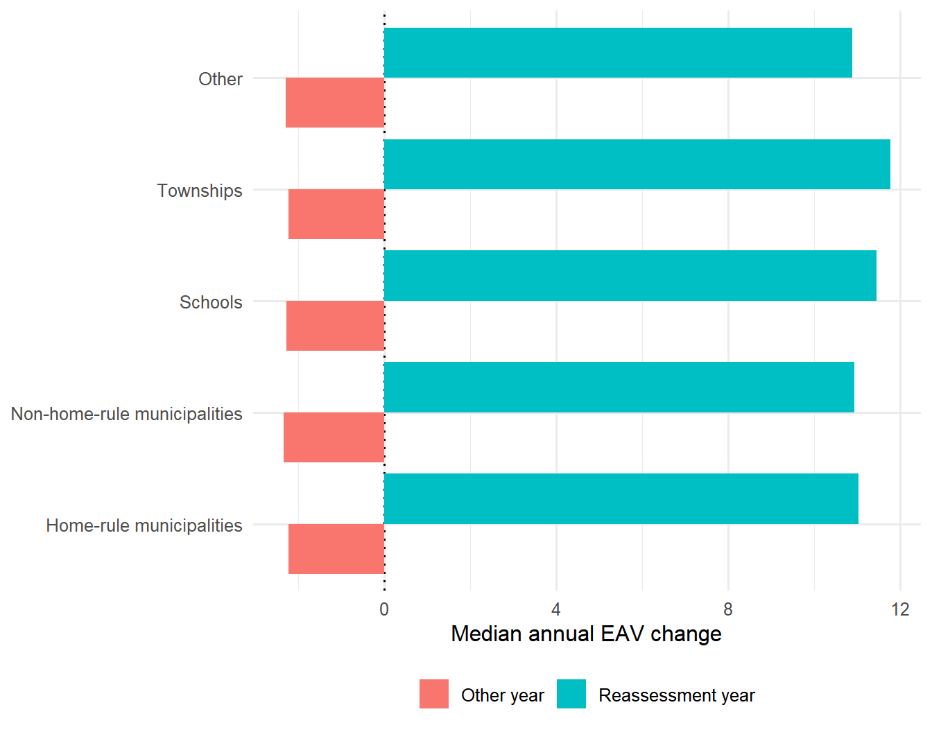
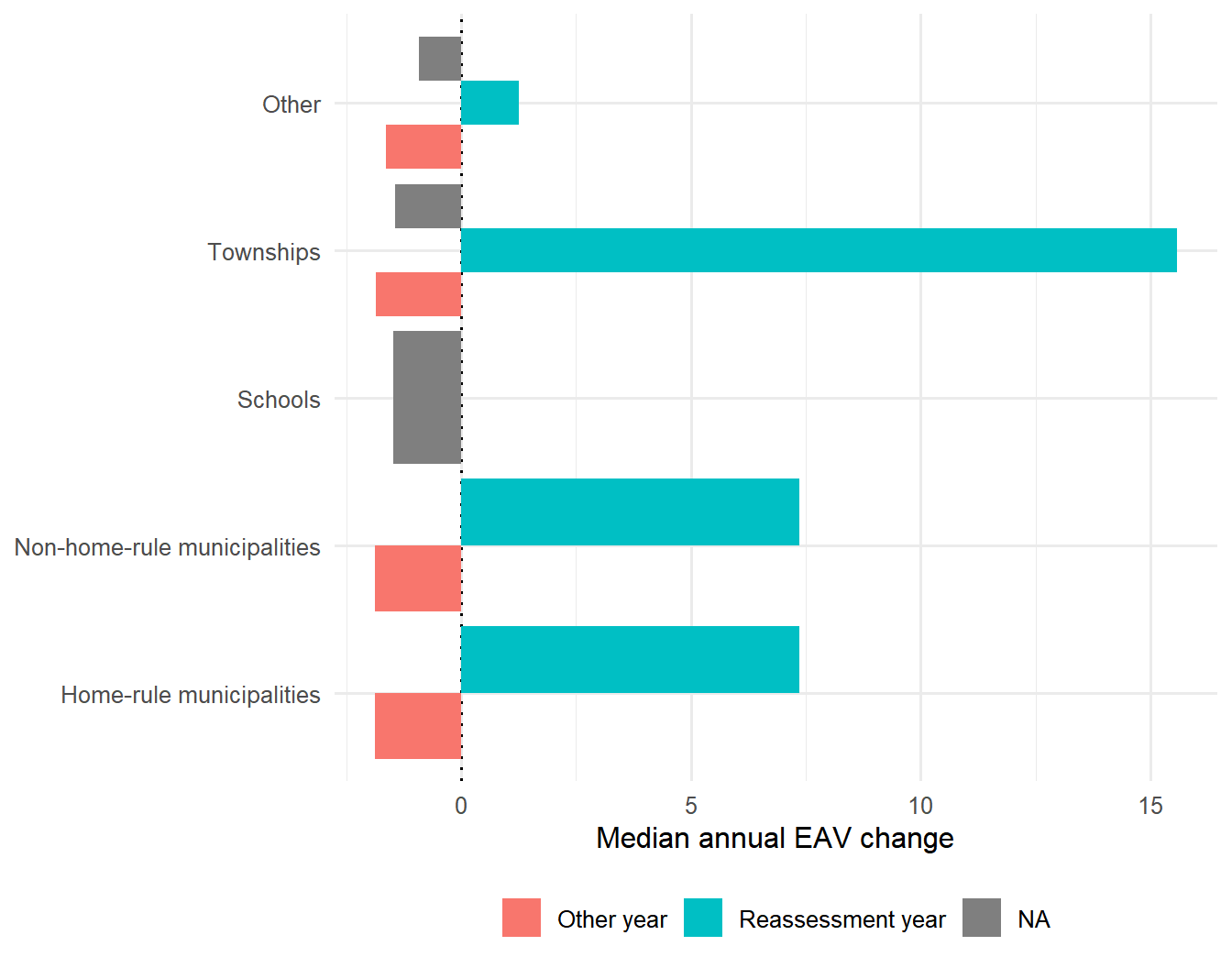
These are descriptive comparisons of instrument relevance, not tests of instrument validity.
::: {.panel-tabset}
## After exclusions
```{r}
#| label: tbl-reassessment-counts-after
#| tbl-cap: "Reassessment-year observations after exclusions"
reassessment_counts_after <- analysis_df |>
  count(agency_type, reassessment_status, name = "Observations") |>
  pivot_wider(names_from = reassessment_status, values_from = Observations, values_fill = 0)

knitr::kable(reassessment_counts_after, align = c("l", "r", "r"))
```
```{r}
#| label: fig-reassessment-after
#| fig-cap: "Median EAV change in reassessment and other years after exclusions"
#| fig-height: 5.5
analysis_df |>
  filter(is.finite(d_eav)) |>
  group_by(agency_type, reassessment_status) |>
  summarise(`Median EAV change` = median(d_eav), .groups = "drop") |>
  ggplot(aes(x = agency_type, y = `Median EAV change`, fill = reassessment_status)) +
  geom_hline(yintercept = 0, linetype = "dotted") +
  geom_col(position = "dodge") +
  coord_flip() +
  labs(x = NULL, y = "Median annual EAV change", fill = NULL) +
  theme(legend.position = "bottom")
```
## Before exclusions
```{r}
#| label: tbl-reassessment-counts-before
#| tbl-cap: "Reassessment-year observations before exclusions"
if (!before_available) {
  cat(before_missing_message)
} else {
  before_change_df |>
    count(agency_type, reassessment_status, name = "Observations") |>
    pivot_wider(names_from = reassessment_status, values_from = Observations, values_fill = 0) |>
    knitr::kable(align = c("l", "r", "r"))
}
```
```{r}
#| label: fig-reassessment-before
#| fig-cap: "Median EAV change in reassessment and other years before exclusions"
#| fig-height: 5.5
if (!before_available) {
  cat(before_missing_message)
} else {
  before_change_df |>
    filter(is.finite(d_eav)) |>
    group_by(agency_type, reassessment_status) |>
    summarise(`Median EAV change` = median(d_eav), .groups = "drop") |>
    ggplot(aes(x = agency_type, y = `Median EAV change`, fill = reassessment_status)) +
    geom_hline(yintercept = 0, linetype = "dotted") +
    geom_col(position = "dodge") +
    coord_flip() +
    labs(x = NULL, y = "Median annual EAV change", fill = NULL) +
    theme(legend.position = "bottom")
}
```
:::
# Long-run growth
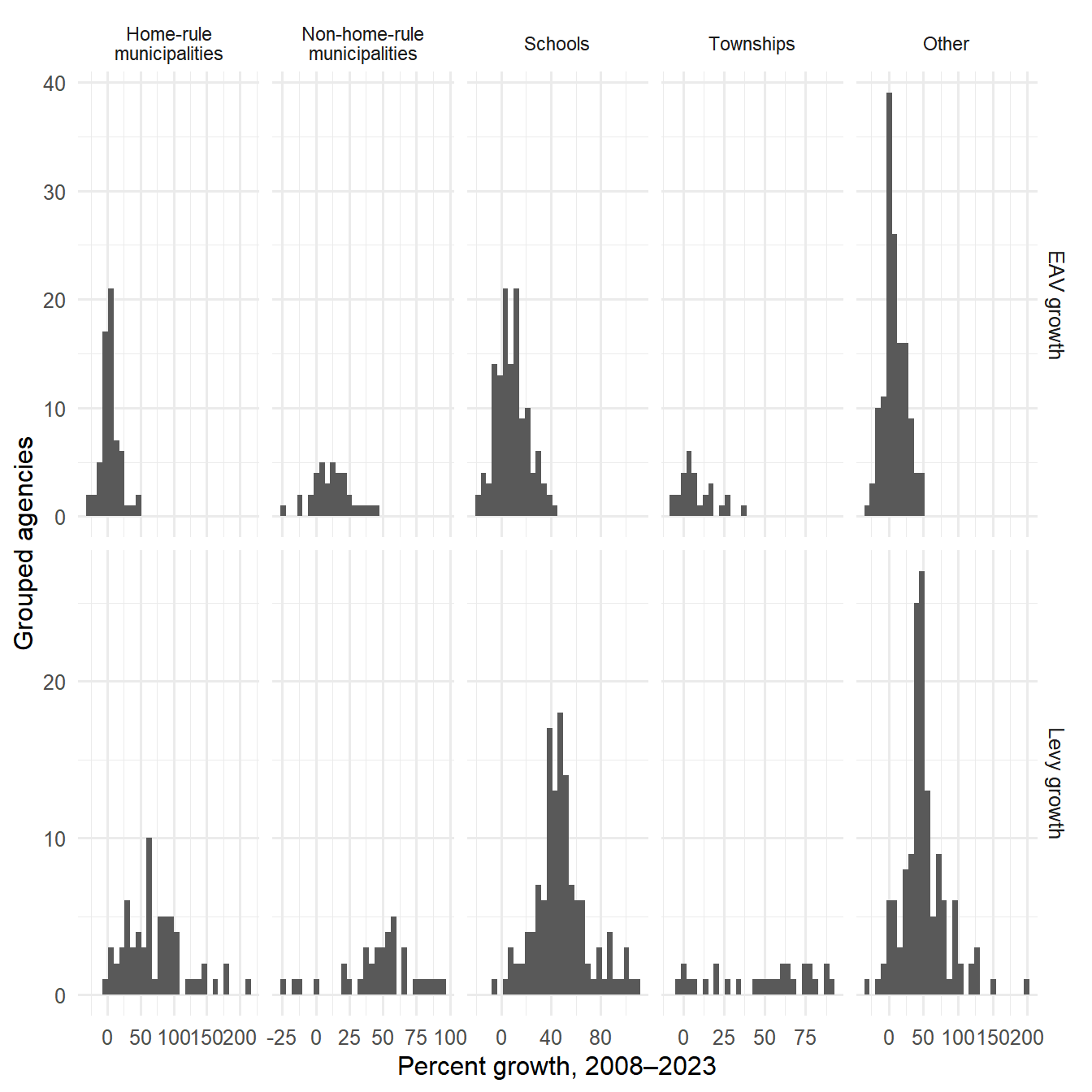
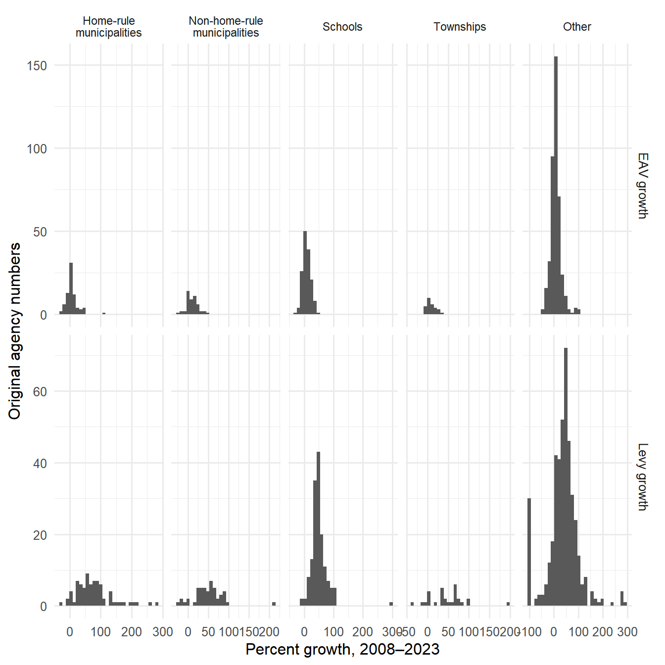
Long-run growth is calculated only for units observed in both `r first_level_year` and `r last_year` with finite endpoint growth rates. Readers can search for an agency or sort the growth columns to identify large increases and declines.
::: {.panel-tabset}
## After exclusions
```{r}
#| label: tbl-long-growth-summary-after
#| tbl-cap: "Long-run levy and EAV growth after exclusions"
long_run_growth_after |>
  group_by(agency_type) |>
  summarise(
    Agencies = n(),
    `Median levy growth (%)` = median(levy_growth),
    `Mean levy growth (%)` = mean(levy_growth),
    `Median EAV growth (%)` = median(eav_growth),
    `Mean EAV growth (%)` = mean(eav_growth),
    .groups = "drop"
  ) |>
  mutate(across(where(is.numeric), ~ round(.x, 1))) |>
  knitr::kable(align = c("l", rep("r", 5)))
```
### Searchable agency-level growth
```{r}
#| label: tbl-agency-growth-after
growth_table_after <- long_run_growth_after |>
  transmute(
    Agency = agency_name_display,
    `Agency type` = as.character(agency_type),
    `Start levy` = start_levy,
    `End levy` = end_levy,
    `Levy growth (%)` = levy_growth,
    `Start EAV` = start_eav,
    `End EAV` = end_eav,
    `EAV growth (%)` = eav_growth,
    `Levy minus EAV growth (percentage points)` = levy_minus_eav_growth
  ) |>
  arrange(desc(`Levy growth (%)`))

DT::datatable(
  growth_table_after,
  rownames = FALSE,
  filter = "top",
  class = "compact stripe hover",
  options = list(
    pageLength = 15,
    lengthMenu = list(
      c(10, 15, 25, 50, 100, -1),
      c("10", "15", "25", "50", "100", "All")
    ),
    order = list(list(4, "desc")),
    scrollX = TRUE,
    autoWidth = TRUE
  )
) |>
  DT::formatCurrency(
    columns = c("Start levy", "End levy", "Start EAV", "End EAV"),
    currency = "$",
    digits = 0,
    mark = ","
  ) |>
  DT::formatRound(
    columns = c(
      "Levy growth (%)",
      "EAV growth (%)",
      "Levy minus EAV growth (percentage points)"
    ),
    digits = 1
  )
```
```{r}
#| label: fig-long-growth-after
#| fig-cap: "Distribution of long-run levy and EAV growth after exclusions"
#| fig-height: 7
long_run_growth_after |>
  select(agency_type, `Levy growth` = levy_growth, `EAV growth` = eav_growth) |>
  pivot_longer(c(`Levy growth`, `EAV growth`), names_to = "Measure", values_to = "Growth") |>
  group_by(Measure) |>
  mutate(
    lower = quantile(Growth, 0.01),
    upper = quantile(Growth, 0.99)
  ) |>
  ungroup() |>
  filter(Growth >= lower, Growth <= upper) |>
  ggplot(aes(x = Growth)) +
  geom_histogram(bins = 30) +
  facet_grid(
    Measure ~ agency_type,
    scales = "free",
    labeller = agency_facet_labeller
  ) +
  labs(
    x = paste0("Percent growth, ", first_level_year, "–", last_year),
    y = "Grouped agencies"
  ) +
  theme(strip.text.x = element_text(size = 8.5))
```
## Before exclusions
```{r}
#| label: tbl-long-growth-summary-before
#| tbl-cap: "Long-run levy and EAV growth before exclusions"
if (!before_available) {
  cat(before_missing_message)
} else {
  long_run_growth_before |>
    group_by(agency_type) |>
    summarise(
      Agencies = n(),
      `Median levy growth (%)` = median(levy_growth),
      `Mean levy growth (%)` = mean(levy_growth),
      `Median EAV growth (%)` = median(eav_growth),
      `Mean EAV growth (%)` = mean(eav_growth),
      .groups = "drop"
    ) |>
    mutate(across(where(is.numeric), ~ round(.x, 1))) |>
    knitr::kable(align = c("l", rep("r", 5)))
}
```
### Searchable agency-level growth
```{r}
#| label: tbl-agency-growth-before
if (!before_available) {
  cat(before_missing_message)
} else {
  growth_table_before <- long_run_growth_before |>
    transmute(
      `Agency number` = agency_id,
      Agency = agency_name_display,
      `Agency type` = as.character(agency_type),
      `Start levy` = start_levy,
      `End levy` = end_levy,
      `Levy growth (%)` = levy_growth,
      `Start EAV` = start_eav,
      `End EAV` = end_eav,
      `EAV growth (%)` = eav_growth,
      `Levy minus EAV growth (percentage points)` = levy_minus_eav_growth
    ) |>
    arrange(desc(`Levy growth (%)`))

  DT::datatable(
    growth_table_before,
    rownames = FALSE,
    filter = "top",
    class = "compact stripe hover",
    options = list(
      pageLength = 15,
      lengthMenu = list(
        c(10, 15, 25, 50, 100, -1),
        c("10", "15", "25", "50", "100", "All")
      ),
      order = list(list(5, "desc")),
      scrollX = TRUE,
      autoWidth = TRUE
    )
  ) |>
    DT::formatCurrency(
      columns = c("Start levy", "End levy", "Start EAV", "End EAV"),
      currency = "$",
      digits = 0,
      mark = ","
    ) |>
    DT::formatRound(
      columns = c(
        "Levy growth (%)",
        "EAV growth (%)",
        "Levy minus EAV growth (percentage points)"
      ),
      digits = 1
    )
}
```
```{r}
#| label: fig-long-growth-before
#| fig-cap: "Distribution of long-run levy and EAV growth before exclusions"
#| fig-height: 7
if (!before_available) {
  cat(before_missing_message)
} else {
  long_run_growth_before |>
    select(agency_type, `Levy growth` = levy_growth, `EAV growth` = eav_growth) |>
    pivot_longer(c(`Levy growth`, `EAV growth`), names_to = "Measure", values_to = "Growth") |>
    group_by(Measure) |>
    mutate(
      lower = quantile(Growth, 0.01),
      upper = quantile(Growth, 0.99)
    ) |>
    ungroup() |>
    filter(Growth >= lower, Growth <= upper) |>
    ggplot(aes(x = Growth)) +
    geom_histogram(bins = 30) +
    facet_grid(
      Measure ~ agency_type,
      scales = "free",
      labeller = agency_facet_labeller
    ) +
    labs(
      x = paste0("Percent growth, ", first_level_year, "–", last_year),
      y = "Original agency numbers"
    ) +
    theme(strip.text.x = element_text(size = 8.5))
}
```
:::
# Data completeness
::: {.panel-tabset}
## After exclusions
```{r}
#| label: tbl-data-completeness-after
#| tbl-cap: "Availability of model variables after exclusions"
analysis_df |>
  group_by(agency_type) |>
  summarise(
    `Agency-year observations` = n(),
    `Finite d_levy` = sum(is.finite(d_levy)),
    `Finite d_eav` = sum(is.finite(d_eav)),
    `Finite d_levy and d_eav` = sum(is.finite(d_levy) & is.finite(d_eav)),
    `Complete IG-revenue change` = sum(!is.na(d_total_ig_revenue)),
    `Complete enrollment change` = sum(!is.na(d_enrollment)),
    .groups = "drop"
  ) |>
  knitr::kable(align = c("l", rep("r", 6)))
```
Enrollment is primarily relevant for school districts, so its missingness for other agency types is structural rather than a general data-quality problem.
## Before exclusions
The original source file does not contain the Census control variables used later in the manuscript. This tab therefore focuses on the availability of levy, EAV, and their annual changes.
```{r}
#| label: tbl-data-completeness-before
#| tbl-cap: "Availability of levy and EAV variables before exclusions"
if (!before_available) {
  cat(before_missing_message)
} else {
  before_change_df |>
    group_by(agency_type) |>
    summarise(
      `Agency-year observations` = n(),
      `Finite levy level` = sum(is.finite(total_final_levy)),
      `Finite EAV level` = sum(is.finite(eav)),
      `Finite d_levy` = sum(is.finite(d_levy)),
      `Finite d_eav` = sum(is.finite(d_eav)),
      `Finite d_levy and d_eav` = sum(is.finite(d_levy) & is.finite(d_eav)),
      .groups = "drop"
    ) |>
    knitr::kable(align = c("l", rep("r", 6)))
}
```
:::
# Optional fund-level appendix
The agency-fund extract is separate from both panel files. This appendix remains disabled so the main descriptive page does not depend on another large data source.
Remove `eval: false` when `agency_funds.csv` is available.
```{r}
#| label: fig-top-fund-names
#| eval: false
#| fig-cap: "Most frequently reported positive-levy fund names in the latest fund-level year"
agency_funds <- readr::read_csv("agency_funds.csv", show_col_types = FALSE)
latest_fund_year <- max(agency_funds$year, na.rm = TRUE)

top_funds <- agency_funds |>
  filter(
    year == latest_fund_year,
    levy > 0,
    major_type != "COOK COUNTY",
    minor_type != "SSA"
  ) |>
  count(fund_name, sort = TRUE, name = "Agencies") |>
  slice_head(n = 15)

top_funds |>
  ggplot(aes(x = reorder(fund_name, Agencies), y = Agencies)) +
  geom_col() +
  coord_flip() +
  labs(
    x = NULL,
    y = "Number of agencies",
    title = paste("Most common fund names in", latest_fund_year)
  )
```