---
title: "Q1 Figures and Tables"
subtitle: "Impact of FEMA designated risk zones on sale price"
format:
html:
df-print: kable
code-fold: true
tbl-cap-location: margin
error: true
toc: true
warning: false
message: false
---
# Setup stuff
```{r setup}
library(tidyverse)
library(fixest)
library(did)
library(etwfe)
library(tidyverse)

library(modelsummary)
library(gt)

options(scipen = 999)

# bldg_sfha <- readRDS("data/processed/variants/df_prep__bldg_sfha.RDS")
#
# parcels <- readRDS("data/processed/variants/df_prep__parcel_sfha.RDS")
#
# bldg_1in500 <- readRDS("data/processed/variants/df_prep__bldg_1in500.RDS")

source("R/helper_pins_to_drop.R")
```
```{r}
lake100ft <- readxl::read_xlsx("data/processed/parcels_2025_lakeMI_within100ft_ExportTable_TableToExcel.xlsx")
lake500ft <- readxl::read_xlsx("data/processed/parcels_2025_lakeMI_within500ft_ExportTable_TableToExcel.xlsx")

bldg_sfha <- readRDS("data/processed/targets/sales/df_prep_bldg_v2026_03.RDS")

parcels <- readRDS("data/processed/targets/sales/df_prep_land_v2026_03.RDS")

bldg_1in500 <- readRDS("data/processed/targets/sales/df_prep_risk500_v2026_03.RDS")  |>
  filter(!pin10 %in% drop_parcels  |
               (pin10 == "0113301013" & sale_year > 2014))

# bldg_sfha <- readRDS("data/processed/variants/df_prep__bldg_sfhaarcgis_redo_2026sales.RDS")
#
# parcels <- readRDS("data/processed/variants/df_prep__parcel_sfhaarcgis_redo_2026sales.RDS")
#
# bldg_1in500 <- readRDS("data/processed/variants/df_prep__bldg_1in500arcgis_redo_2026sales.RDS") |>
#   filter(!pin10 %in% drop_parcels  |
#            (pin10 == "0113301013" & sale_year > 2014))


bldg_sfha <- bldg_sfha |> filter(!pin10 %in% drop_parcels  |
               (pin10 == "0113301013" & sale_year > 2014)
             )

parcels <- parcels |> filter(!pin10 %in% drop_parcels  |
               (pin10 == "0113301013" & sale_year > 2014)
             )

make_control_groups <- function(df,
                                ever_added,
                                ever_removed,
                    pre_eff_change_type,
                    type = c("pre", "eff")
                                ){

  # Treated Group A: Added to Risk Zone
  group_T_A <- df |>
    filter( {{ever_added}} == TRUE )

  # Treated Group B: Removed from Risk Zone
  group_T_B <- df |>
      filter( {{ever_removed}}  == TRUE)

  # Control Group A:  Never in SFHA, FIRM panels never updated

   if(type == "pre"){
   group_C_A <- df |>
      filter(
        {{pre_eff_change_type}} == "Never SFHA" &
             pre_date_chr %in% c("2005-01-01")
         )
  }else if(type == "eff"){  # for effective maps
  group_C_A <- df |>
      filter(
        {{pre_eff_change_type}} == "Never SFHA" &
         eff_date_chr %in% c("2008-08-19")
         )
  }

    # Control Group B: Never in SFHA, FIRM Panels are updated
    group_C_B  <- df |>
      filter(
        {{pre_eff_change_type}} == "Never SFHA" &
         (eff_date_chr %in% c("2019-11-01", "2021-09-10") |
             pre_date_chr %in% c("2015-02-12", "2019-07-01", "2021-09-22")
         )
         )

    # Control Group C: Always in SFHA, FIRM Panels are not updated
    if(type == "pre"){
    group_C_C <- df |>
      filter(
        {{pre_eff_change_type}} == "Always SFHA" &
          pre_date_chr %in% c("2005-01-01")
      )}
    else if(type == "eff") {  # this probably is tainted by prelim map cohort in 2021 though....
    group_C_C <- df |>
      filter(
        {{pre_eff_change_type}} == "Always SFHA" &
         (eff_date_chr %in% c("2008-08-19") )
      )

    group_C_C_alt <- df |>
      filter(
        {{pre_eff_change_type}} == "Always SFHA" &
         (eff_date_chr %in% c("2008-08-19") |
            pre_date_chr %in% c("2005-01-01")
          )
      )
    }

    # Always in SFHA but FIRM panels have been recently updated

    if(type == "eff") {
      group_C_D <- df |>
        filter(
        {{pre_eff_change_type}} == "Always SFHA" &
         (eff_date_chr %in% c("2019-11-01", "2021-09-10"))
         )

       group_C_D_alt <- df |>
        filter(
        {{pre_eff_change_type}} == "Always SFHA" &
         (eff_date_chr %in% c("2019-11-01", "2021-09-10") |
             pre_date_chr %in% c("2015-02-12", "2019-07-01", "2021-09-22")
             )
         )
    } else if (type == "pre") {
      group_C_D <- df |>
         filter(
        {{pre_eff_change_type}} == "Always SFHA" &
             pre_date_chr %in% c("2015-02-12", "2019-07-01", "2021-09-22")
         )
    }
      list(
    group_T_A = group_T_A,
    group_T_B = group_T_B,
    group_C_A = group_C_A,
    group_C_B = group_C_B,
    group_C_C = group_C_C,
    group_C_D = group_C_D

  )

}

groups <- make_control_groups(df = bldg_sfha,
                    ever_added = ever_added_prelim,
                    ever_removed = ever_removed_prelim,
                    pre_eff_change_type = change_type_prelim,
                    type = "pre")

groups_long <- imap_dfr(groups, ~ {
  .x |>
    mutate(group = .y)
})
```
```{r}
groups_long |>
  group_by(group) |>
  summarise(
    n = n(),
    n_properties = n_distinct(pin),
    mean_price = mean(sale_price, na.rm = TRUE),
    mean_log_price = mean(log_price, na.rm = TRUE)
  )
```
## Line Graphs
```{r }
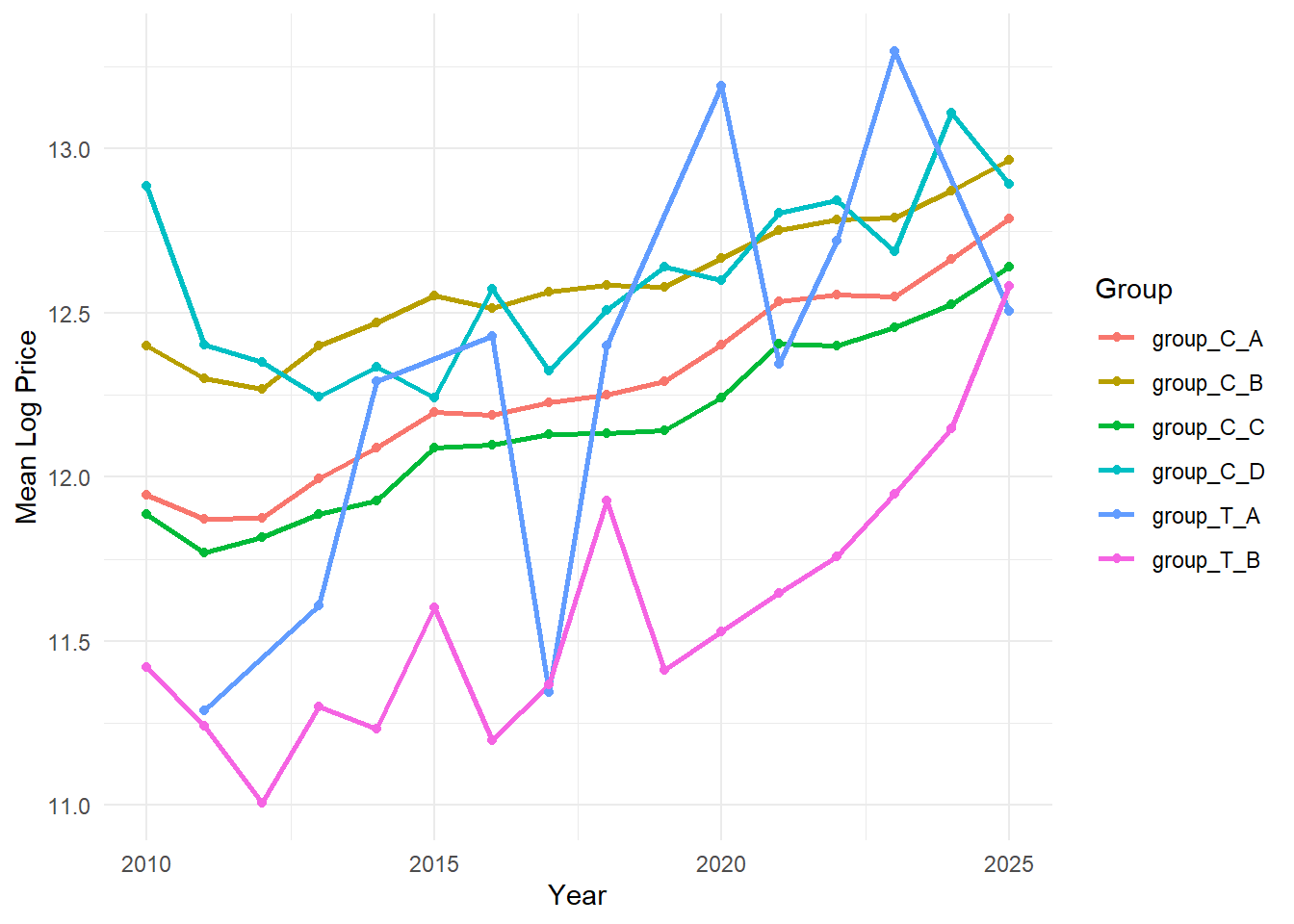
group_trends <- groups_long |>
  group_by(group, sale_year) |>
  summarise(
    mean_log_price = mean(log_price, na.rm = TRUE),
    n = n(),
    .groups = "drop"
  )

ggplot(group_trends, aes(x = sale_year, y = mean_log_price, color = group)) +
  geom_line(linewidth = 1) +
  geom_point(size = 1.5) +
  labs(
    x = "Year",
    y = "Mean Log Price",
    color = "Group"
  ) +
  theme_minimal()
```
```{r}
#| layout-ncol: 2
groups_long <- groups_long |>
  mutate(group_type = case_when(
    group %in% c("group_T_A", "group_T_B") ~ "Treated",
    TRUE ~ "Control"
  ))

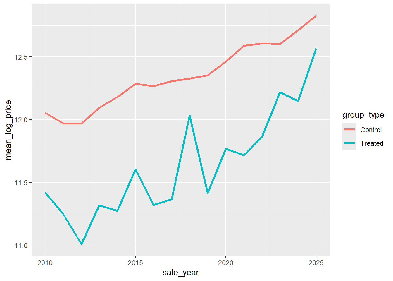
group_trends2 <- groups_long |>
  group_by(group_type, sale_year) |>
  summarise(
    mean_log_price = mean(log_price, na.rm = TRUE),
    .groups = "drop"
  )

ggplot(group_trends2, aes(x = sale_year, y = mean_log_price, color = group_type)) +
  geom_line(linewidth = 1.2)
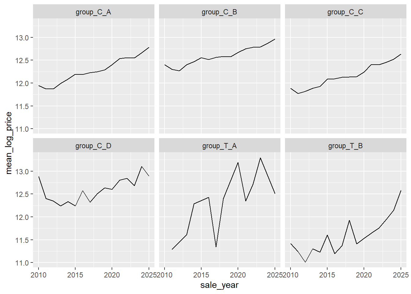
ggplot(group_trends, aes(x = sale_year, y = mean_log_price)) +
  geom_line() +
  facet_wrap(~ group)
```
# Question 1
## Table 2: Sample Counts
```{r}
table(bldg_sfha$prelim_sfha_category)
table(bldg_sfha$change_type_prelim)
table(bldg_sfha$eff_sfha_category)
table(bldg_sfha$change_type)
```
```{r}
df_es_added <- bldg_sfha |>
  filter(pin10 %in% groups$group_T_A$pin10 | pin10 %in% groups$group_C_B$pin10 )|>
 # filter(prelim_sfha_category %in% c("Added to prelim SFHA", "Never SFHA")) |>
  mutate(pin_num = as.numeric(pin)) |>
  dplyr::arrange(pin_num, sale_year, sale_date) |>
  dplyr::group_by(pin_num, sale_year, pre_date_chr) |>
  dplyr::slice_tail(n = 1) |>
  dplyr::ungroup() |>
  mutate(treated = prelim_sfha_category == "Added to prelim SFHA") |>

   group_by(pin_num) |>
  mutate(
    g_add = if (any(addedto_prelim_sfha == 1, na.rm = TRUE)) {
      min(sale_year[addedto_prelim_sfha == 1], na.rm = TRUE)
    } else {
      0L
    }
  ) |>
  ungroup()


added_counts <- table(df_es_added$g_add, df_es_added$pre_date)


df_es_removed <- bldg_sfha |>
    filter(pin10 %in% groups$group_T_B$pin10 | pin10 %in% groups$group_C_D$pin10 )|>

  #filter(prelim_sfha_category %in% c("Removed from prelim SFHA", "Always SFHA")) |>
  mutate(pin_num = as.numeric(pin)) |>
  dplyr::arrange(pin_num, sale_year, sale_date) |>
  dplyr::group_by(pin_num, sale_year, pre_date_chr) |>
  dplyr::slice_tail(n = 1) |>
  dplyr::ungroup() |>
  mutate(treated = prelim_sfha_category == "Removed from prelim SFHA") |>

   group_by(pin_num) |>
  mutate(
    g_remove = if (any(removedfrom_prelim_sfha == TRUE, na.rm = TRUE)) {
      min(sale_year[removedfrom_prelim_sfha == TRUE], na.rm = TRUE)
    } else {
      0L
    }
  ) |>
  ungroup()


removed_counts <- table(df_es_removed$g_remove, df_es_removed$pre_date)
```
```{r}
#| label: tbl-table1-treatedsalesbycohort
#| tbl-cap: "Table 1: Treated Sales by Cohort and Treatment Direction"
#| layout-ncol: 2
added_counts
removed_counts
```
## Table 3
```{r}
#| label: tbl-table3-descriptivestatsforQ1
#| tbl-cap: "Table3: Descriptive Statistics for Sample"
sfha_category_stats <- bldg_sfha |>
  group_by(pin) |> mutate(n_sales = n()) |> ungroup() |>
  group_by(change_type_prelim) |>
 summarize(
    n_properties = n_distinct(pin),
    avg_sales_per_property = mean(n_sales),
    n_sales      = n(),
    avg_price = mean(sale_price),
    median_price = median(sale_price)  ) |>
  arrange(desc(n_properties))

sfha_category_stats
sfha_category_stats <- bldg_sfha |>
    mutate(ever_firm_update =  ifelse(pre_date =="2005-01-01", FALSE, TRUE) ) |>
  group_by(change_type_prelim) |>
  filter(ever_firm_update==TRUE) |>
  summarize(
    n_properties = n_distinct(pin),
    avg_sales_per_property = mean(n_sales),
    n_sales      = n(),
    avg_price = mean(sale_price),
    median_price = median(sale_price)  ) |>
  arrange(desc(n_properties))

sfha_category_stats
sfha_category_stats <- bldg_sfha |>
  group_by(prelim_sfha_category) |>
  summarize(
    n_properties = n_distinct(pin),
    avg_sales_per_property = mean(n_sales),
    n_sales      = n(),
    avg_price = mean(sale_price),
    median_price = median(sale_price)  ) |>
  arrange(desc(n_properties))

sfha_category_stats
sfha_category_stats <- bldg_sfha |>
    mutate(ever_firm_update =  ifelse(pre_date =="2005-01-01", FALSE, TRUE) ) |>
  group_by(prelim_sfha_category) |>
  filter(ever_firm_update==TRUE) |>
  summarize(
    n_properties = n_distinct(pin),
    avg_sales_per_property = mean(n_sales),
    n_sales      = n(),
    avg_price = mean(sale_price),
    median_price = median(sale_price)  ) |>
  arrange(desc(n_properties))

sfha_category_stats
```
```{r}
#| label: fig-figure5
#| layout-ncol: 2
allsales_bldg_sfha <- readRDS("data/processed/targets/sales/allsales_bldg_v2026_03.RDS")


allsales_bldg_sfha <- allsales_bldg_sfha |>
  filter(!pin10 %in% c("0122400028", "0516106013"))|>
  filter(!(Triad != "City" & log_price > 13.5))
```
```{r}
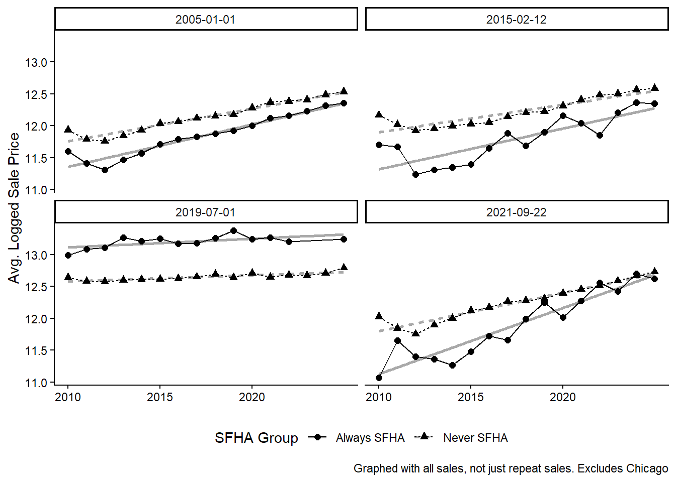
#| label: fig-figure5-cohorttrends
#| fig-cap:
#| - "Includes Chicago"
#| - "Excludes Chicago"
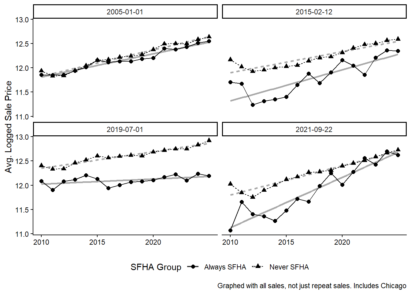
allsales_bldg_sfha |>
  filter(!pin10 %in% c("0122400028", "0516106013")) |> #filter(log_price > 13.5)|>
  filter(prelim_sfha_category %in% c("Always SFHA", "Never SFHA")) |>
    group_by(sale_year, prelim_sfha_category, pre_date_chr) |>
  summarise(avg_logprice = mean(log_price, na.rm = TRUE) )|>

  ggplot(aes(x = sale_year , y = avg_logprice, shape = prelim_sfha_category)) +
  theme_classic() +
  theme(legend.position = "bottom")+
  geom_smooth(aes(lty = prelim_sfha_category), method = "lm", se = FALSE, color = "darkgray", alpha= 0.5, lwd = 1) +
  geom_line(aes(lty = prelim_sfha_category)) +
  geom_point(size = 2) +

  scale_x_continuous(breaks = c(2010, 2015, 2020, 2026)) +
  labs(#title = "Cohort Trends by SFHA Group: Always In vs. Always Out",
       #subtitle = "Includes Chicago",
       y = "Avg. Logged Sale Price",
       x = NULL,
              shape = "SFHA Group",
       lty = "SFHA Group",
              caption = "Graphed with all sales, not just repeat sales. Includes Chicago") +
  facet_wrap(~pre_date_chr)

# EXCLUDE CHCICGO
allsales_bldg_sfha |>
  filter(!pin10 %in% c("0122400028", "0516106013")) |> filter(Triad != "City")|>
  filter(prelim_sfha_category %in% c("Always SFHA", "Never SFHA")) |>
    group_by(sale_year, prelim_sfha_category, pre_date_chr) |>
  summarise(avg_logprice = mean(log_price, na.rm = TRUE) )|>

  ggplot(aes(x = sale_year , y = avg_logprice, shape = prelim_sfha_category)) +
  theme_classic() +
  theme(legend.position = "bottom")+
  geom_smooth(aes(lty = prelim_sfha_category), method = "lm", se = FALSE, color = "darkgray", alpha= 0.5, lwd = 1) +
  geom_line(aes(lty = prelim_sfha_category)) +
  geom_point(size = 2) +

  scale_x_continuous(breaks = c(2010, 2015, 2020, 2026)) +
  labs(#title = "Cohort Trends by SFHA Group: Always In vs. Always Out",
       #subtitle = "Excludes Chicago",
       y = "Avg. Logged Sale Price",
       x = NULL,
              shape = "SFHA Group",
       lty = "SFHA Group",
       caption = "Graphed with all sales, not just repeat sales. Excludes Chicago") +
  facet_wrap(~pre_date_chr)
```
```{r}
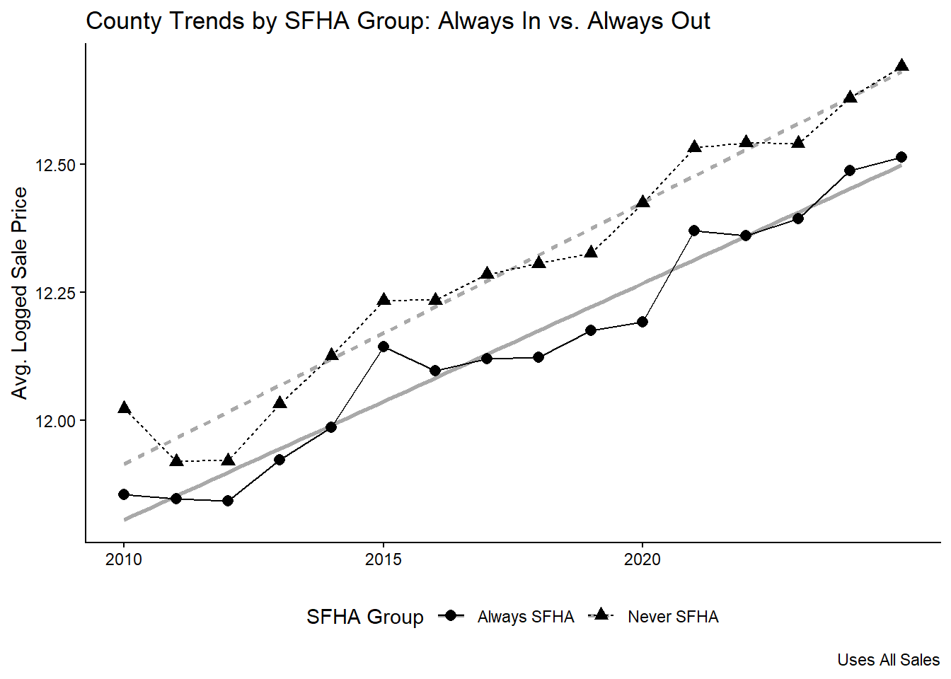
#| label: fig-figure6
#| fig-label: "Figure 6"
allsales_bldg_sfha |>
   filter(!pin10 %in% c("0122400028", "0516106013")) |>
  #filter(!(Triad != "City" & log_price > 13.5))|>
  filter(prelim_sfha_category %in% c("Always SFHA", "Never SFHA")) |>
    group_by(sale_year, prelim_sfha_category) |>
  summarise(avg_logprice = mean(log_price, na.rm = TRUE) )|>

  ggplot(aes(x = sale_year , y = avg_logprice, shape = prelim_sfha_category)) +
  theme_classic() +
  theme(legend.position = "bottom")+
  geom_smooth(aes(lty = prelim_sfha_category), method = "lm", se = FALSE, color = "darkgray", alpha= 0.5, lwd = 1) +
  geom_line(aes(lty = prelim_sfha_category)) +
  geom_point(size = 2.5) +

  scale_x_continuous(breaks = c(2010, 2015, 2020, 2026)) +
  labs(title = "County Trends by SFHA Group: Always In vs. Always Out",
       y = "Avg. Logged Sale Price",
       x = NULL,
       caption= "Uses All Sales",
              shape = "SFHA Group",
       lty = "SFHA Group")
```
## Table 4: County Wide Effect
```{r }
#| label: tbl-table4-prelim-countywide
#| tbl-cap: "Table 4"
bldg_sfha <- bldg_sfha |>
  mutate(nbhd_code = if_else(
    is.na(nbhd_code),
    "Missing",
    as.character(nbhd_code)
  ))

mods <- list (
 no_fe <- feols(
    log_price ~ in_prelim_sfha,
    vcov = ~pin10,
    data = bldg_sfha
  ),

 one_fe <- feols(
    log_price ~ in_prelim_sfha | sale_year,
    data = bldg_sfha,
     vcov = ~pin10
  ),
   pin_fe <- feols(
    log_price ~ in_prelim_sfha | pin ,
    data = bldg_sfha,
        vcov = ~pin10,

  ),

  two_fe <- feols(
    log_price ~ in_prelim_sfha | pin + sale_year,
    data = bldg_sfha,
     vcov = ~pin10
  ),

  three_fe <- feols(
    log_price ~ in_prelim_sfha | pin + sale_year + qtr,
    data = bldg_sfha,
     vcov = ~pin10
)
)
# mod_prelim_3fe <- feols(
#   log_price ~ in_prelim_sfha | pin + sale_year + qtr,
#   data = bldg_sfha
# )
#
# mod_eff_3fe <- feols(
#   log_price ~ in_eff_sfha | pin + sale_year + qtr,
#   data = bldg_sfha
# )
#
# mods_names <- list(
#   "Preliminary"      = mod_prelim,
#   "Effective"        = mod_eff
#   # , "Prelim w/ Qtr FE" = mod_prelim_3fe,
#   #"Eff w/ Qtr FE"    = mod_eff_3fe
# )
#
# vcovs <- list(
#   "Parcel" = ~pin10,
#   "Municipality" = ~clean_name
#   # , "Neighborhood" = ~nbhd_code
# )
#
# gof_labels <- c(
#   "nobs"      = "Observations",
#   "r.squared" = "R-squared"
# )

coef_labels = c(
  "in_prelim_sfhaTRUE" = "In SFHA (Preliminary Map)",
  "in_eff_sfhaTRUE"    = "In SFHA (Effective Map)"
)

# ms_models <- list()
# ms_vcov   <- list()
#
# for (m in names(mods)) {
#   for (v in names(vcovs)) {
#     ms_models[[paste(m, v, sep = "\n")]] <- mods[[m]]
#     ms_vcov[[length(ms_vcov) + 1]] <- vcovs[[v]]
#   }
# }
#
# modelsummary::modelsummary(
#   ms_models,
#   vcov = ms_vcov,
#   stars = TRUE,
#
# )

modelsummary::modelsummary(
  mods,
  stars = TRUE,
 gof_omit = "IC|Log|Adj|Within"
#  ,
 # estimate = "{estimate}{stars}",
#  statistic = "\n({std.error})"#,
,  coef_map = coef_labels
)
```
```{r }
#| label: table4-prelim-countywide-robustnesschecks
#| tbl-cap: "Table 4 robustness check"
modelsummary::modelsummary(
  mods,
  stars = TRUE,
 gof_omit = "IC|Log|Adj|Within",
vcov = ~clean_name
,  coef_map = coef_labels
)
modelsummary::modelsummary(
  mods,
  stars = TRUE,
 gof_omit = "IC|Log|Adj|Within",
vcov = ~nbhd_code
,  coef_map = coef_labels
)
```
## Table 5: Simple Directional Effects - Standard TWFE
```{r}
#| label: tbl-table5-simple-effectofremapping
#| tbl-cap: "Table 5: Effect of Being Mapped Into or Out of a FEMA Flood Plain"
prelim_twfe <- list(


 "I" =  feols(
    log(sale_price) ~ addedto_prelim_sfha  | pin + sale_year,
    cluster = ~pin10,
        data = bldg_sfha
  ),

  "II" =  feols(
    log(sale_price) ~ removedfrom_prelim_sfha | pin + sale_year,
    cluster = ~ pin10,
        data = bldg_sfha,

  ),

  # Asymmetric: added vs removed in one equation
  "0" = feols(
    log(sale_price) ~ addedto_prelim_sfha + removedfrom_prelim_sfha | pin + sale_year,
    cluster = ~ pin10,
        data = bldg_sfha,
  ))


all_models_formatted <- modelsummary::modelsummary(prelim_twfe,
               output = "flextable",
               fmt = function(x) round(x, 2),

             stars = TRUE)

all_models_formatted
```
## Table 5 & 6: Directional Effects & Control Group Subsamples
```{r}
#| label: tbl-effectofremapping
#| tbl-cap: "**Table 5 & 6** Effect of Being Mapped Into or Out of a FEMA Flood Plain. A lot of models all by each other."
#| error: true
##| eval: false

prelim_twfe <- list(


 "I" =  feols(
    log(sale_price) ~ addedto_prelim_sfha  | pin + sale_year,
    cluster = ~pin10,
        data = bldg_sfha
  ),

    "I Subset" = feols(
    log(sale_price) ~ addedto_prelim_sfha  | pin + sale_year,
    cluster = ~ pin10,
        data = (bldg_sfha |> filter(change_type_prelim != "Always SFHA" & treat_year_remove_prelim == 10000)),

  ),

  "II" =  feols(
    log(sale_price) ~ removedfrom_prelim_sfha | pin + sale_year,
    cluster = ~ pin10,
        data = bldg_sfha,

  ),


  "II Subset" =  feols(
    log(sale_price) ~ removedfrom_prelim_sfha | pin + sale_year,
    cluster = ~ pin10,
        data = (bldg_sfha |> filter(change_type_prelim != "Never SFHA" & treat_year_add_prelim == 10000)),

  ),

  # Symmetric effect of location in risk zone
    "Symmetric" = feols(
    log(sale_price) ~ in_prelim_sfha | pin + sale_year,
    cluster = ~ pin10,
        data = bldg_sfha,
  ),

  # Asymmetric: added vs removed in one equation
  "0" = feols(
    log(sale_price) ~ addedto_prelim_sfha + removedfrom_prelim_sfha | pin + sale_year,
    cluster = ~ pin10,
        data = bldg_sfha,
  )
)

all_models_formatted <- modelsummary::modelsummary(prelim_twfe,
               output = "flextable",
               fmt = function(x) round(x, 2),

             stars = TRUE)

all_models_formatted
```
## Table 7: Restrict Samples - Updated FIRM Panels only
```{r}
#| label: tbl-table-7-subset-removedfrom
#| tbl-cap: "**Table 7:** Mapped out of Preliminary SFHA - Restricted Samples"
#|
# function with default options:
fn_valid_cohorts <- function(df){

  df |>
    mutate(pre_date_chr = as.character(pre_date_chr)) |>
    group_by(pre_date_chr) |>
    summarise(
      n = n(),
      n_treated = sum(removedfrom_prelim_sfha == TRUE, na.rm = TRUE),
      n_untreated = sum(removedfrom_prelim_sfha == FALSE, na.rm = TRUE),
          .groups = "drop"

      ) |>
    filter(n_treated > 0,  n_untreated > 0) |>
    pull(pre_date_chr)
}


#table(bldg_sfha$Triad, bldg_sfha$prelim_sfha_category)

df_sub <- bldg_sfha |>
      filter(pin10 %in% groups$group_T_B$pin10 | pin10 %in% groups$group_C_D$pin10 )
  # filter(change_type_prelim != "Never SFHA" &
  #          # and properties that are never treated for being added to the SFHA
  #          treat_year_add_prelim == 10000 & treat_year_add_eff == 10000)

valid_cohorts_bldg <- fn_valid_cohorts(df_sub)
bldgs_fsplit <- df_sub |> filter(pre_date_chr %in% valid_cohorts_bldg)


#table(parcels$Triad, parcels$prelim_sfha_category)
#table(parcels$removed_pre_thisyear, parcels$year)

# df_sub_parcels <- parcels |>
#       filter(pin10 %in% groups$group_T_B$pin10 | pin10 %in% groups$group_C_D$pin10 )
#   # filter(change_type_prelim != "Never SFHA" &
#   #          # and properties that are never treated for being added to the SFHA
#   #          treat_year_add_prelim == 10000 & treat_year_add_eff == 10000)
#
# valid_cohorts_parcels <- fn_valid_cohorts(df = df_sub_parcels)
# parcels_fsplit <- df_sub_parcels |> filter(pre_date_chr %in% valid_cohorts_parcels)
#
# table(bldg_1in500$removed_pre_thisyear, bldg_1in500$year)
# table(bldg_1in500$removedfrom_prelim_sfha, bldg_1in500$year)
# table(bldg_1in500$Triad, bldg_1in500$prelim_sfha_category)
# df_sub_1in500 <- bldg_1in500 |>
#   filter(change_type_prelim != "Never SFHA" &
#            # and properties that are never treated for being added to the SFHA
#            treat_year_add_prelim == 10000 & treat_year_add_eff == 10000)
# valid_cohorts_1in500 <- fn_valid_cohorts(df = df_sub_1in500)
# bldg_1in500_fsplit <- df_sub_1in500 |> filter(pre_date_chr %in% valid_cohorts_1in500)
#
#


models <- list(
 "Bldg SFHA" = feols(
       log(sale_price) ~ removedfrom_prelim_sfha | pin + sale_year,

   # log(sale_price) ~ event_remapped*ever_removed_prelim | pin + sale_year,
    data = bldgs_fsplit,
  fsplit = ~pre_date_chr,
    cluster = ~pin10
  )
  #
  # "Bldg 1in500" = feols(
  #          log(sale_price) ~ removedfrom_prelim_sfha | pin + sale_year,
  #
  # #  log(sale_price) ~ event_remapped*ever_removed_prelim | pin + sale_year,
  #   data = bldg_1in500_fsplit,
  # fsplit = ~pre_date_chr,
  #   cluster = ~pin10
  #
  # ),
  #
  # "Parcels" = feols(
  #          log(sale_price) ~ removedfrom_prelim_sfha | pin + sale_year,
  #
  # #  log(sale_price) ~ event_remapped*ever_removed_prelim | pin + sale_year,
  #   data = parcels_fsplit,
  # fsplit = ~pre_date_chr,
  #   cluster = ~pin10
  #
  # )
)

all_models_formatted <- modelsummary::modelsummary(models,
               output = "flextable",
               fmt = function(x) round(x, 2),

             stars = TRUE)

all_models_formatted
```
## Table 8
```{r}
#| label: tbl-table8-subset-prelim_addedto
#| tbl-cap: "Table 8: Mapped into Preliminary SFHA - Restricted Sample"
#|
#table(bldg_sfha$added_pre_thisyear, bldg_sfha$year)

# function with default options:
fn_valid_cohorts <- function(df){

  df |>
    mutate(pre_date_chr = as.character(pre_date_chr)) |>
    group_by(pre_date_chr) |>
    summarise(
      n = n(),
      n_treated = sum(addedto_prelim_sfha == TRUE, na.rm = TRUE),
      n_untreated = sum(addedto_prelim_sfha == FALSE, na.rm = TRUE),
          .groups = "drop"

      ) |>
    filter(n_treated > 0,  n_untreated > 0) |>
    pull(pre_date_chr)
}


table(bldg_sfha$Triad, bldg_sfha$prelim_sfha_category)
df_sub <- bldg_sfha |>
    filter(pin10 %in% groups$group_T_A$pin10 | pin10 %in% groups$group_C_B$pin10 )
  # filter(change_type_prelim != "Always SFHA" &
  #          # and properties that are never treated for being removed from the SFHA
  #          treat_year_remove_prelim == 10000 & treat_year_remove_eff == 10000)

valid_cohorts_bldg <- fn_valid_cohorts(df_sub)
bldgs_fsplit <- df_sub |> filter(pre_date_chr %in% valid_cohorts_bldg)


# table(parcels$Triad, parcels$prelim_sfha_category)
# table(parcels$removed_pre_thisyear, parcels$year)

df_sub_parcels <- parcels |>
    filter(pin10 %in% groups$group_T_A$pin10 | pin10 %in% groups$group_C_B$pin10 )
  # filter(change_type_prelim != "Always SFHA" &
  #          # and properties that are never treated for being removed from the SFHA
  #          treat_year_remove_prelim == 10000 & treat_year_remove_eff == 10000)
valid_cohorts_parcels <- fn_valid_cohorts(df = df_sub_parcels)
parcels_fsplit <- df_sub_parcels |> filter(pre_date_chr %in% valid_cohorts_parcels)


#
# table(bldg_1in500$removed_pre_thisyear, bldg_1in500$year)
# table(bldg_1in500$removedfrom_prelim_sfha, bldg_1in500$year)
# table(bldg_1in500$Triad, bldg_1in500$prelim_sfha_category)

# df_sub_1in500 <- bldg_1in500 |>
#     filter(pin10 %in% groups$group_T_A$pin10 | pin10 %in% groups$group_C_B$pin10 )
  # filter(change_type_prelim != "Always SFHA" &
  #          # and properties that are never treated for being removed from the SFHA
  #          treat_year_remove_prelim == 10000 & treat_year_remove_eff == 10000)
#valid_cohorts_1in500 <- fn_valid_cohorts(df = df_sub_1in500)
#bldg_1in500_fsplit <- df_sub_1in500 |> filter(pre_date_chr %in% valid_cohorts_1in500)


models_pre_add <- list(
  # Heterogeneity by Triad: added/removed interacted with Triad
  #
  # # Heterogeneity by Triad: added/removed interacted with Triad
  "Buildings in SFHA" =  feols(
    log(sale_price) ~ addedto_prelim_sfha | pin + sale_year,
    fsplit = ~pre_date_chr,
    cluster = ~pin10,
    data = bldgs_fsplit
  ),
    "Buildings in SFHA" =  feols(
    log(sale_price) ~ addedto_prelim_sfha*condo | pin + sale_year,
    fsplit = ~pre_date_chr,
    cluster = ~pin10,
    data = bldgs_fsplit
  ),

  "Buildings in SFHA" =  feols(
    log(sale_price) ~ addedto_prelim_sfha | pin + sale_year,
    cluster = ~pin10,
    data = bldg_sfha
  )
  #
  # "Buildings - 1-in-500" =  feols(
  #   log(sale_price) ~ addedto_prelim_sfha | pin + year,
  #   fsplit = ~pre_date_chr,
  #   cluster = ~pin10,
  #   data = bldg_1in500_fsplit
  # ),
  #
  # "Buildings - 1-in-500" =  feols(
  #   log(sale_price) ~ addedto_prelim_sfha | pin + sale_year,
  #   cluster = ~pin10,
  #   data = bldg_1in500
  # )
)

all_models_formatted <- modelsummary::modelsummary(models_pre_add,
                                                   output = "flextable",
                                                   fmt = function(x) round(x, 2),

                                                   stars = TRUE)

all_models_formatted
```
## Table 9: County-wide and Cohort Directional Models using Extended TWFE
### Added To Risk Zone
```{r}
#| label: tbl-table9-column1-extwfe-with-groups-withchicago
#| tbl-cap: "Control Groups A, B, C, & D (so all PINs that never changed SFHA status; both always in, and always out)"
mod1c = etwfe(
  fml = log_price ~ 1,
  tvar = sale_year,
  ivar = pin,
  cgroup = "never",
  gvar = treat_year_add_prelim,
  vcov = ~pin10,
  data = (bldg_sfha |>
            filter(
             (pin %in% groups$group_T_A$pin |
              pin %in% groups$group_C_A$pin |
              pin %in% groups$group_C_B$pin |
              pin %in% groups$group_C_C$pin |
              pin %in% groups$group_C_D$pin )
                     )
          )
  )
# mod1c
emfx(mod1c)
emfx(mod1c, type = "group")
```
```{r}
#| label: test-table-with-groups-withchicago
#| tbl: "Includes Chicago Observations. Control Groups A & B"
#| eval: false
#| include: false
mod1c = etwfe(
fml = log_price ~ 1,
tvar = sale_year,
ivar = pin,
cgroup = "never",
gvar = treat_year_add_prelim,
vcov = ~pin10,
data = (bldg_sfha |>
filter(
(pin %in% groups$group_T_A$pin |
pin %in% groups$group_C_A$pin |
pin %in% groups$group_C_B$pin )
)
)
)
mod1c
emfx(mod1c)
emfx(mod1c, type = "group")
```
### Mapped Out of SFHA, Column 3
```{r table9-column3}
mod2 = etwfe(
  fml = log_price ~ 1,
  tvar = sale_year,
  ivar = pin,
  cgroup = "never",
  gvar = treat_year_remove_prelim,
  vcov = ~pin10,
  data = (bldg_sfha|>
                filter(pin10 %in% groups$group_T_B$pin10 |
                         pin10 %in% groups$group_C_D$pin10 |
                         pin10 %in% groups$group_C_C$pin10 |
                         pin10 %in% groups$group_C_A$pin10 |
                         pin10 %in% groups$group_C_B$pin10 )

          )
  )
# mod2
emfx(mod2)
emfx(mod2, type = "group")
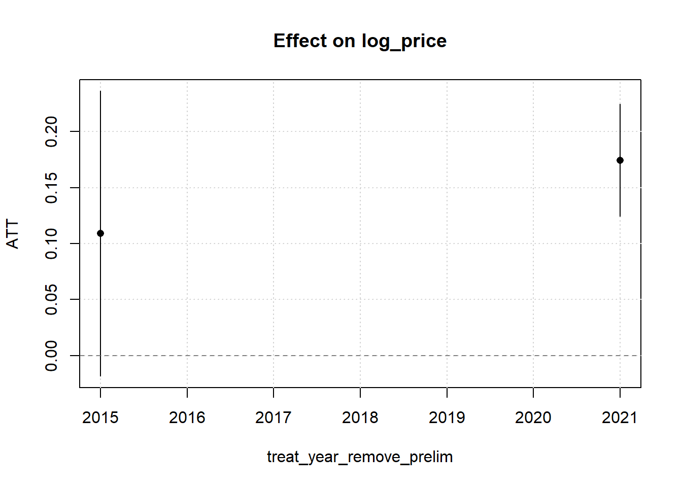
plot(emfx(mod2, type = "group"))
```
### Removed - Subset (Column 4)
```{r}
mod2 = etwfe(
  fml = log_price ~ 1,
  tvar = sale_year,
  ivar = pin,
  cgroup = "never",
  gvar = treat_year_remove_prelim,
  vcov = ~pin10,
  data = (bldg_sfha|>
                filter(pin10 %in% groups$group_T_B$pin10 |
                         pin10 %in% groups$group_C_D$pin10 |
                         pin10 %in% groups$group_C_C$pin10 )

          )
  )
# mod2
emfx(mod2)
emfx(mod2, type = "group")
#plot(emfx(mod2, type = "group"))
```
## Table 10: Regional Slopes
### Mapped into SFHA
```{r table10-column1-regional-slopes}
library(etwfe)

mod1 = etwfe(
  fml = log_price ~ 1,
  tvar = sale_year,
  ivar = pin,
  xvar = Triad,
  cgroup = "never",
  gvar = treat_year_add_prelim,
  vcov = ~pin10,
  data = (bldg_sfha |>
            filter(treat_year_remove_prelim==10000

                   & change_type_prelim != "Always SFHA")
          )

  )
#mod1
emfx(mod1)
emfx(mod1, type = "group")
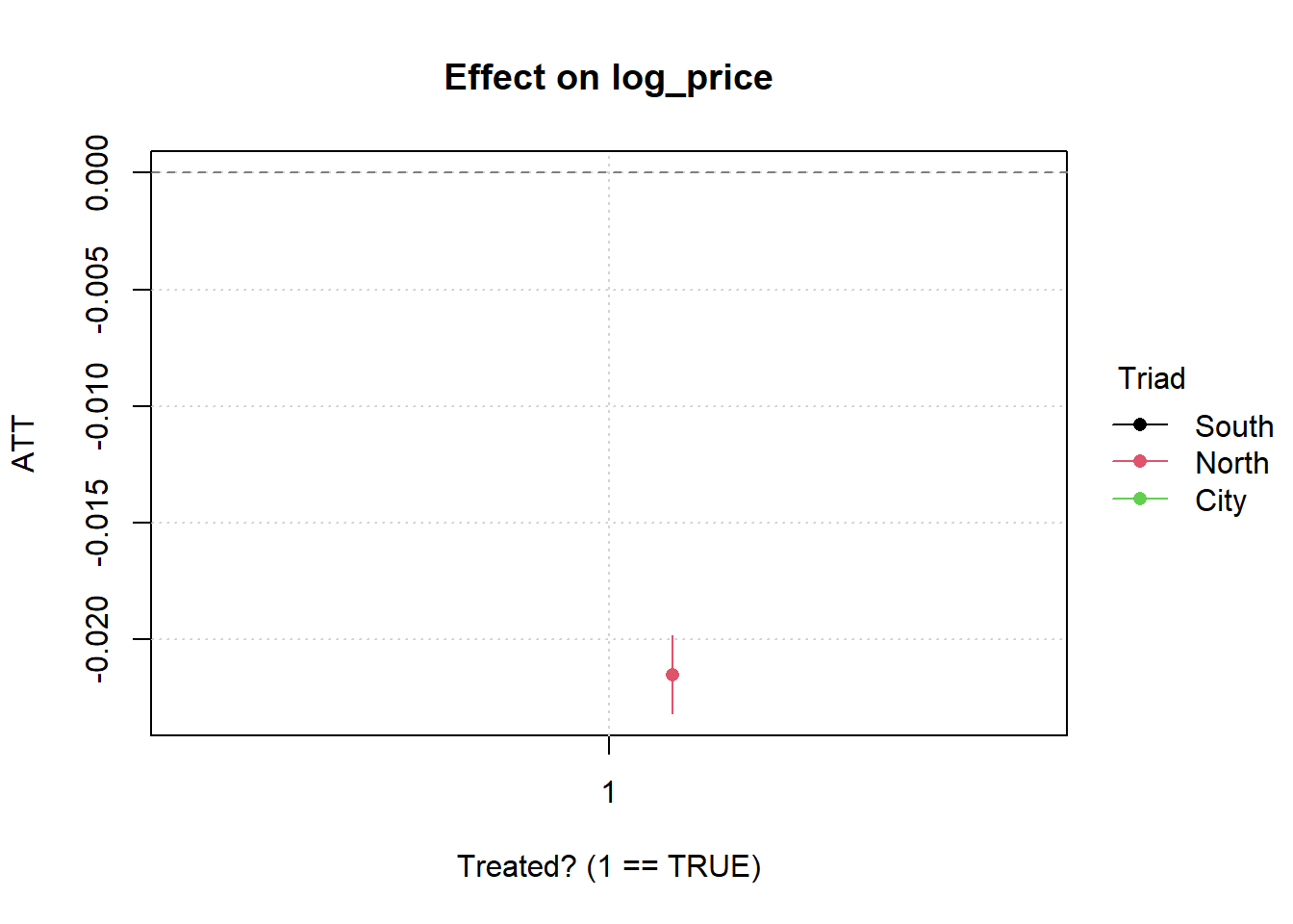
plot(emfx(mod1))
```
### Added with regional slopes
```{r table10-column1}
mod2 = etwfe(
  fml = log_price ~ 1,
  tvar = sale_year,
  ivar = pin,
  cgroup = "never",
  gvar = treat_year_add_prelim,
    xvar = Triad,

  vcov = ~pin10,
  data = (bldg_sfha|>
                filter(pin10 %in% groups$group_T_A$pin10 |
                         pin10 %in% groups$group_C_A$pin10 |
                         pin10 %in% groups$group_C_B$pin10)
          )
  )
# mod2
emfx(mod2)
emfx(mod2, type = "group")
```
```{r table10-column2}
mod2 = etwfe(
  fml = log_price ~ 1,
  tvar = sale_year,
  ivar = pin,
  cgroup = "never",
  gvar = treat_year_add_prelim,
  xvar = group_name_prelim,
  vcov = ~pin10,
  data = (bldg_sfha|>
                filter(pin10 %in% groups$group_T_A$pin10 |
                         pin10 %in% groups$group_C_A$pin10 |
                         pin10 %in% groups$group_C_B$pin10
                         )
          )
  )
# mod2
emfx(mod2)
emfx(mod2, type = "group")
```
```{r table10-column3}
mod2 = etwfe(
  fml = log_price ~ 1,
  tvar = sale_year,
  ivar = pin,
  cgroup = "never",
  gvar = treat_year_remove_prelim,
    xvar = Triad,

  vcov = ~pin10,
  data = (bldg_sfha|>
                filter(pin10 %in% groups$group_T_B$pin10 |
                         pin10 %in% groups$group_C_D$pin10 |
                         pin10 %in% groups$group_C_C$pin10
                         )
          )
  )
# mod2
#emfx(mod2)
emfx(mod2, type = "group")
```
```{r table10-column4}
mod2 = etwfe(
  fml = log_price ~ 1,
  tvar = sale_year,
  ivar = pin,
  cgroup = "never",
  gvar = treat_year_remove_prelim,
  xvar = group_name_prelim,

  vcov = ~pin10,
  data = (bldg_sfha|>
                filter(pin10 %in% groups$group_T_B$pin10 |
                         pin10 %in% groups$group_C_D$pin10 |
                         pin10 %in% groups$group_C_C$pin10
                         )
          )
  )
# mod2
emfx(mod2)
emfx(mod2, type = "group")
```
```{r}
#| label: tbl-table11-effectiveSFHA-subset-removed
#| tbl-cap: "Table 11: Mapped out of EFFECTIVE SFHA - Restricted Sample"
#|
#table(bldg_sfha$added_pre_thisyear, bldg_sfha$year)

# function with default options:
fn_valid_cohorts <- function(df){

  df |>
    mutate(eff_date_chr = as.character(eff_date_chr)) |>
    group_by(eff_date_chr) |>
    summarise(
      n = n(),
      n_treated = sum(removedfrom_eff_sfha == TRUE, na.rm = TRUE),
      n_untreated = sum(removedfrom_eff_sfha == FALSE, na.rm = TRUE),
          .groups = "drop"

      ) |>
    filter(n_treated > 0,  n_untreated > 0) |>
    pull(eff_date_chr)
}


df_sub <- bldg_sfha |>
      filter(pin10 %in% groups$group_T_B$pin10 | pin10 %in% groups$group_C_D$pin10 )
  # filter(change_type_prelim != "Never SFHA" &
  #          # and properties that are never treated for being addedto from the SFHA
  #          treat_year_add_prelim == 10000 & treat_year_add_eff == 10000)

valid_cohorts_bldg <- fn_valid_cohorts(df_sub)
bldgs_fsplit <- df_sub |> filter(eff_date_chr %in% valid_cohorts_bldg)


# table(parcels$Triad, parcels$prelim_sfha_category)
# table(parcels$removed_pre_thisyear, parcels$year)

df_sub_parcels <- parcels |>
      filter(pin10 %in% groups$group_T_B$pin10 | pin10 %in% groups$group_C_D$pin10 )
  # filter(change_type_prelim != "Never SFHA" &
  #          # and properties that are never treated for being added to the SFHA
  #          treat_year_add_prelim == 10000 & treat_year_add_eff == 10000)
valid_cohorts_parcels <- fn_valid_cohorts(df = df_sub_parcels)
parcels_fsplit <- df_sub_parcels |> filter(eff_date_chr %in% valid_cohorts_parcels)


#
# table(bldg_1in500$removed_pre_thisyear, bldg_1in500$year)
# table(bldg_1in500$removedfrom_prelim_sfha, bldg_1in500$year)
# table(bldg_1in500$Triad, bldg_1in500$prelim_sfha_category)

df_sub_1in500 <- bldg_1in500 |>
      filter(pin10 %in% groups$group_T_B$pin10 | pin10 %in% groups$group_C_D$pin10 )
  # filter(change_type_prelim != "Never SFHA" &
  #          # and properties that are never treated for being addedto the SFHA
  #          treat_year_add_prelim == 10000 & treat_year_add_eff == 10000)
valid_cohorts_1in500 <- fn_valid_cohorts(df = df_sub_1in500)
bldg_1in500_fsplit <- df_sub_1in500 |> filter(eff_date_chr %in% valid_cohorts_1in500)


models <- list(

  # "Buildings in SFHA" =  feols(
  #   log(sale_price) ~ addedto_eff_sfha | pin + sale_year,
  #   fsplit = ~eff_date_chr,
  #   cluster = ~pin10,
  #   data = bldgs_fsplit
  # ),

  "Buildings in SFHA" =  feols(
    log(sale_price) ~ removedfrom_eff_sfha | pin + sale_year,
    fsplit = ~eff_date_chr,

    cluster = ~pin10,
    data = parcels_fsplit
  ),

  "Buildings - 1-in-500" =  feols(
    log(sale_price) ~ removedfrom_eff_sfha | pin + year,
    fsplit = ~eff_date_chr,
    cluster = ~pin10,
    data = bldg_1in500_fsplit
  )
)

all_models_formatted <- modelsummary::modelsummary(models,
                                                   output = "flextable",
                                                   fmt = function(x) round(x, 2),

                                                   stars = TRUE)

all_models_formatted
```
```{r}
#| label: table11-effectiveSFHA-subset-addedto
#| tbl-cap: "Table 11: Mapped into EFFECTIVE SFHA - Restricted Sample"
#|
#table(bldg_sfha$added_pre_thisyear, bldg_sfha$year)

# function with default options:
fn_valid_cohorts <- function(df){

  df |>
    mutate(eff_date_chr = as.character(eff_date_chr)) |>
    group_by(eff_date_chr) |>
    summarise(
      n = n(),
      n_treated = sum(addedto_eff_sfha == TRUE, na.rm = TRUE),
      n_untreated = sum(addedto_eff_sfha == FALSE, na.rm = TRUE),
          .groups = "drop"

      ) |>
    filter(n_treated > 0,  n_untreated > 0) |>
    pull(eff_date_chr)
}


table(bldg_sfha$Triad, bldg_sfha$prelim_sfha_category)
df_sub <- bldg_sfha |>
  filter(change_type_prelim != "Always SFHA" &
           # and properties that are never treated for being removed from the SFHA
           treat_year_remove_prelim == 10000 & treat_year_remove_eff == 10000)

valid_cohorts_bldg <- fn_valid_cohorts(df_sub)
bldgs_fsplit <- df_sub |> filter(eff_date_chr %in% valid_cohorts_bldg)


# table(parcels$Triad, parcels$prelim_sfha_category)
# table(parcels$removed_pre_thisyear, parcels$year)

df_sub_parcels <- parcels |>
  filter(change_type_prelim != "Always SFHA" &
           # and properties that are never treated for being removed from the SFHA
           treat_year_remove_prelim == 10000 & treat_year_remove_eff == 10000)
valid_cohorts_parcels <- fn_valid_cohorts(df = df_sub_parcels)
parcels_fsplit <- df_sub_parcels |> filter(eff_date_chr %in% valid_cohorts_parcels)


#
# table(bldg_1in500$removed_pre_thisyear, bldg_1in500$year)
# table(bldg_1in500$removedfrom_prelim_sfha, bldg_1in500$year)
# table(bldg_1in500$Triad, bldg_1in500$prelim_sfha_category)

df_sub_1in500 <- bldg_1in500 |>
  filter(change_type != "Always SFHA" &
           # and properties that are never treated for being removed from the SFHA
           treat_year_remove_prelim == 10000 & treat_year_remove_eff == 10000)
valid_cohorts_1in500 <- fn_valid_cohorts(df = df_sub_1in500)
bldg_1in500_fsplit <- df_sub_1in500 |> filter(eff_date_chr %in% valid_cohorts_1in500)


models <- list(

  # "Buildings in SFHA" =  feols(
  #   log(sale_price) ~ addedto_eff_sfha | pin + sale_year,
  #   fsplit = ~eff_date_chr,
  #   cluster = ~pin10,
  #   data = bldgs_fsplit
  # ),

  "Buildings in SFHA" =  feols(
    log(sale_price) ~ addedto_eff_sfha | pin + sale_year,
    cluster = ~pin10,
    data = bldg_sfha
  ),

  "Buildings - 1-in-500" =  feols(
    log(sale_price) ~ addedto_eff_sfha | pin + year,
    fsplit = ~eff_date_chr,
    cluster = ~pin10,
    data = bldg_1in500_fsplit
  ),

  "Buildings - 1-in-500" =  feols(
    log(sale_price) ~ addedto_eff_sfha | pin + sale_year,
    cluster = ~pin10,
    data = bldg_1in500
  )
)

all_models_formatted <- modelsummary::modelsummary(models,
                                                   output = "flextable",
                                                   fmt = function(x) round(x, 2),

                                                   stars = TRUE)

all_models_formatted
```
## Table 11: Countywide Effective Map Dates
```{r}
eff_twfe = list(
 "I-Eff" =  feols(
    log(sale_price) ~ addedto_eff_sfha  | pin + sale_year,
    cluster = ~ pin10,
        data = bldg_sfha
  ),

    "I-Eff Subset" = feols(
    log(sale_price) ~ addedto_eff_sfha  | pin + sale_year,
    cluster = ~ pin10,
        data = (bldg_sfha |> filter(change_type != "Always SFHA" & treat_year_remove_eff == 10000)),

  ),

  "II-Eff" =  feols(
    log(sale_price) ~ removedfrom_eff_sfha | pin + sale_year,
    cluster = ~ pin10,
        data = bldg_sfha,

  ),


  "II-Eff Subset" =  feols(
    log(sale_price) ~ removedfrom_eff_sfha | pin + sale_year,
    cluster = ~ pin10,
        data = bldg_sfha |> filter(change_type != "Never SFHA" & treat_year_add_prelim == 10000),

  ),

  # Symmetric effect of location in risk zone
    "III-Eff" = feols(
    log(sale_price) ~ in_eff_sfha | pin + sale_year,
    cluster = ~ pin10,
        data = bldg_sfha,

  ),
  # Asymmetric: added vs removed in one equation
  "0-Eff" = feols(
    log(sale_price) ~ addedto_eff_sfha + removedfrom_eff_sfha | pin + sale_year,
    cluster = ~ pin10,
        data = bldg_sfha,

  )
 )
all_models_formatted <- modelsummary::modelsummary(eff_twfe,
               output = "flextable",
               fmt = function(x) round(x, 2),

             stars = TRUE)

all_models_formatted
```
```{r}
#| label: tbl-table11-effective-countywide
#| tbl-cap: "Table 11"
mods <- list (
 no_fe <- feols(
    log_price ~ in_eff_sfha,
    vcov = ~pin10,
    data = bldg_sfha
  ),

 one_fe <- feols(
    log_price ~ in_eff_sfha | sale_year,
    data = bldg_sfha,
     vcov = ~pin10
  ),
pin_fe <- feols(
    log_price ~ in_eff_sfha | pin ,
    data = bldg_sfha,
        vcov = ~pin10,
  ),

  two_fe <- feols(
    log_price ~ in_eff_sfha | pin + sale_year,
    data = bldg_sfha,
     vcov = ~pin10
  ),

  three_fe <- feols(
    log_price ~ in_eff_sfha | pin + sale_year + qtr,
    data = bldg_sfha,
     vcov = ~pin10
)
)


coef_labels = c(
  "in_prelim_sfhaTRUE" = "In SFHA (Preliminary Map)",
  "in_eff_sfhaTRUE"    = "In SFHA (Effective Map)"
)

modelsummary::modelsummary(
  mods,
  stars = TRUE,
 gof_omit = "IC|Log|Adj|Within"
,  coef_map = coef_labels
)
```
```{r}
#| label: table-11-effective-countywide-robustnesschecks
#| tbl-cap: "Table 11 robustness checks"
#| layout-ncol: 2
#| eval: false
#| include: false
modelsummary::modelsummary(
mods,
stars = TRUE,
gof_omit = "IC|Log|Adj|Within",
vcov = ~clean_name
, coef_map = coef_labels
)
modelsummary::modelsummary(
mods,
stars = TRUE,
gof_omit = "IC|Log|Adj|Within",
vcov = ~nbhd_code
, coef_map = coef_labels
)
```
## Alternative exposure definitions: conventional TWFE {#q1-spatial-definitions}
This section supports the page-56 reference to alternative spatial identifiers and Tables XIII-XIV. The saved grid compares building-footprint and parcel-based SFHA exposure with the two corresponding 1-in-500-year exposure variants. Preliminary and effective map timing appear in separate columns. The 1-in-500-year variants represent the broader flood-exposure definition used by their source datasets; their exact geometry and inclusion rules should be read with the spatial-processing code.
The conventional TWFE grid is loaded from `outputs/tables/grid_tbl_twfe.rds`, written by `Q1_Model_Comparison.qmd`. Its rows distinguish specifications and addition/removal indicators; cells show estimates and standard errors with significance markers. Changes across columns may reflect both classification and sample differences. The grid's correspondence to individual printed table cells remains to be reconciled; it should not be treated as a new estimation run.
```{r}
source("R/q1_grid_html.R")
read_q1_grid_html("outputs/tables/grid_tbl_twfe.rds")
```
## Alternative exposure definitions: extended TWFE {#q1-spatial-etwfe}
This grid loads `outputs/tables/grid_tbl_etwfe.rds`, assembled by `etwfe_combined_mega_grid.qmd` from saved preliminary/effective model results. It reports countywide, triad, or cohort aggregations as labeled, across the four exposure definitions. These aggregations differ from the conventional coefficient grid above. The source file contains both general and no-Chicago result paths; the precise saved-grid sample must be reconciled before claiming an exact replication of Table XIV.
```{r}
read_q1_grid_html("outputs/tables/grid_tbl_etwfe.rds")
```
### Treated-observation inventory {#q1-exposure-counts}
The small number of treated properties discussed around dissertation page 56 can vary sharply with the exposure definition. This inventory uses the four current `df_prep_*_v2026_03` exports and the project's manual parcel exclusions. It counts post-transition sales and distinct 10-digit parcels separately for preliminary/effective additions/removals. These are input-sample counts, not the effective estimation sample of every model in the saved grids: missing variables, fixed-effect singleton removal, control-group restrictions, and geographic exclusions can change a fitted model's sample. They should not be labeled as exact dissertation table counts until reconciled with the original fitted models.
```{r}
#| label: q1-exposure-count-inventory
q1_exposure_paths <- c(
  `Building - SFHA` = "data/processed/targets/sales/df_prep_bldg_v2026_03.RDS",
  `Parcel - SFHA` = "data/processed/targets/sales/df_prep_land_v2026_03.RDS",
  `Building - 1-in-500` = "data/processed/targets/sales/df_prep_risk500_v2026_03.RDS",
  `Parcel - 1-in-500` = "data/processed/targets/sales/df_prep_risk500_land_v2026_03.RDS"
)
q1_exposure_counts <- purrr::imap_dfr(q1_exposure_paths, function(path, definition) {
  if (!file.exists(path)) stop("Missing exposure dataset: ", path)
  d <- readRDS(path) |>
    dplyr::filter(!pin10 %in% drop_parcels | (pin10 == "0113301013" & sale_year > 2014))
  indicators <- c(
    `Preliminary: added` = "addedto_prelim_sfha",
    `Preliminary: removed` = "removedfrom_prelim_sfha",
    `Effective: added` = "addedto_eff_sfha",
    `Effective: removed` = "removedfrom_eff_sfha"
  )
  if (!all(c("pin10", unname(indicators)) %in% names(d))) {
    stop("Missing transition identifiers in ", path)
  }
  purrr::imap_dfr(indicators, function(variable, transition) {
    flag <- as.character(d[[variable]])
    if (!all(stats::na.omit(flag) %in% c("TRUE", "FALSE", "1", "0"))) {
      stop("Unexpected transition coding in ", path, ": ", variable)
    }
    treated <- !is.na(flag) & flag %in% c("TRUE", "1")
    tibble::tibble(
      Definition = definition, Transition = transition,
      `Input sales` = nrow(d), `Treated sales` = sum(treated),
      `Treated parcels` = dplyr::n_distinct(d$pin10[treated], na.rm = TRUE),
      `Missing transition flag` = sum(is.na(flag))
    )
  })
})
knitr::kable(q1_exposure_counts, caption = "Current input-sample treatment counts by exposure definition")
```
# Appendix A: Q1 research-design assumptions {#appendix-a}
This section supports the Appendix A reference on dissertation page 35 and the discussion on printed pages 91-99. It examines pretreatment trends, possible anticipation, and sensitivity to outcome scale and regional controls. The event studies below use preliminary-map timing and distinguish additions from removals; they are not a diagnostic for every effective-map or alternative-exposure specification elsewhere on the site.
| Supporting item | Location |
|---|---|
| Event studies, individual leads, and joint pretrend tests | [Additions](#q1-added-event-study) and [removals](#q1-removed-event-study) |
| Extended-TWFE event profiles | [Existing event-profile output](#q1-etwfe-event-profiles) |
| Two-year-early placebo tests | [Placebo results](#q1-placebo-tests) |
| Conditional parallel trends | [Regional-control comparison](#q1-conditional-trends) |
| Levels, logs, inverse price, and inverse hyperbolic sine | [Transformation comparison](#q1-outcome-transformations) |
| Historical distributional diagnostics | [Saved results and provenance](#q1-distributional-tests) |
The regional and transformation comparisons are newly assembled supporting outputs. Existing event-study and placebo formulas are retained. Saved distributional diagnostics come from older samples and are identified separately. No diagnostic alone proves the causal assumptions.
[Return to the dissertation index](index.qmd#page-35-question-1-research-design-assumptions).
## Additions: event study and pretrend tests {#q1-added-event-study}
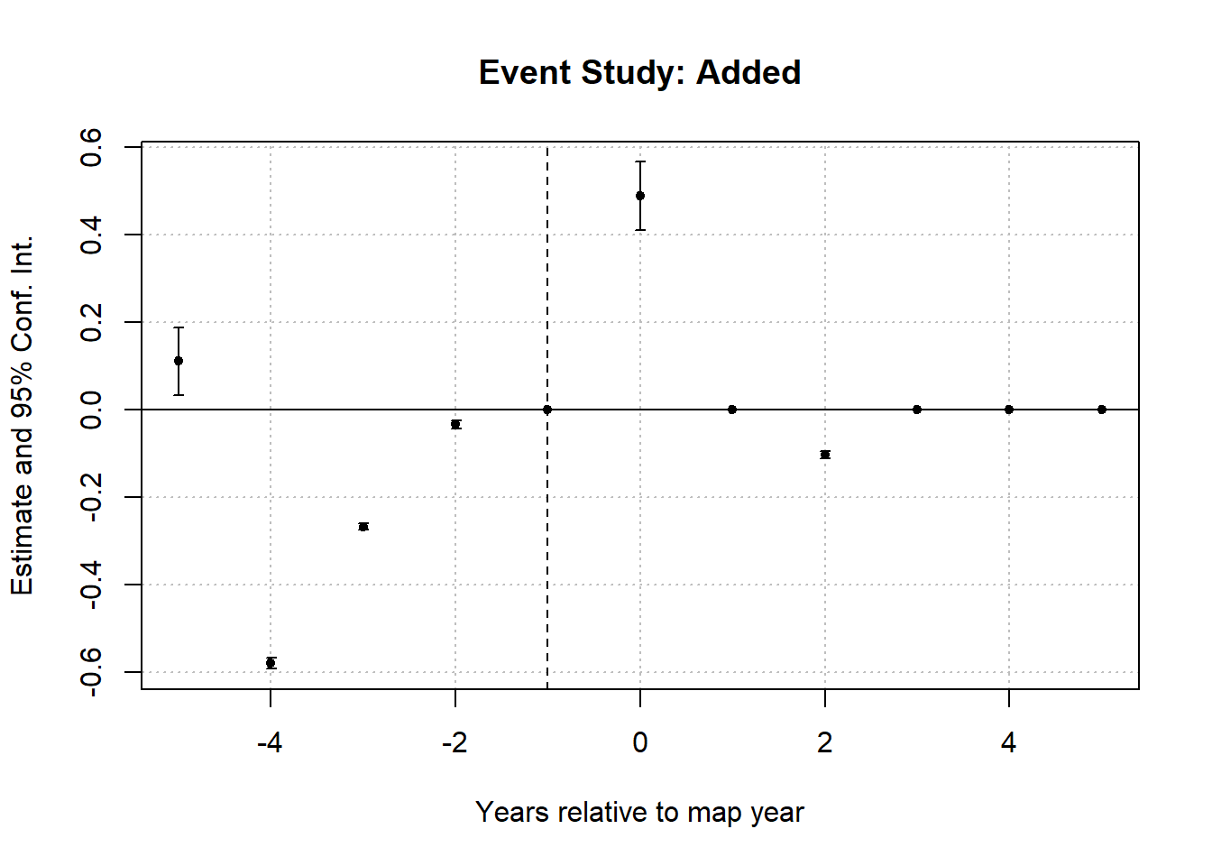
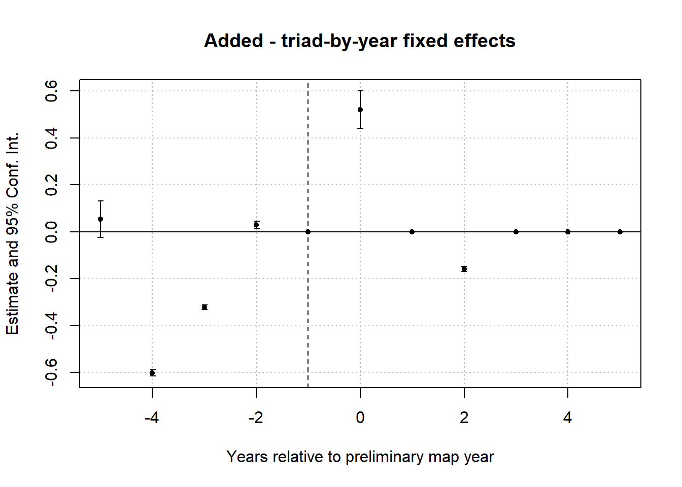
Properties added to the preliminary SFHA are compared with never-SFHA properties. Event time is relative to the preliminary map year; sales earlier than the preliminary date within that year are assigned to year -1. The endpoint bins pool years at or below -5 and at or above +5. Year -1 is the omitted reference period.
The plotted model uses logged sale price, property and year fixed effects, and standard errors clustered by 10-digit parcel. The coefficient table below the plot lists estimated pretreatment leads; the Wald test jointly tests the included leads -5 through -2 against zero relative to year -1. Rejection raises concerns about the specification or pre-event comparability. Non-rejection is not proof of parallel trends, especially when treated samples are small.
```{r}
out_dir <- "outputs/q2_marginaleffects"
prep_path <- file.path(out_dir, "bldg_sfha_q2_dissertation_prepped.rds")
if (!file.exists(prep_path)) {
  source("scripts/q2_dissertation_scripts/q2_dissertation_00_prep_data.R")
}

bldg_sfha <- readRDS(prep_path)

df_prep <- bldg_sfha |>
  mutate(
    pre_year = if ("pre_year" %in% names(bldg_sfha)) pre_year else as.integer(format(pre_date, "%Y")),
    eff_year = if ("eff_year" %in% names(bldg_sfha)) eff_year else as.integer(format(eff_date, "%Y")),
    event_time = sale_year - pre_year,
    event_time = ifelse(event_time == 0 & sale_date < pre_date, -1, event_time)
  )

# ----  bin leads/lags ----
df_prep <- df_prep |>
  mutate(
    event_time_binned = case_when(
      event_time <= -5 ~ -5L,
      event_time >=  5 ~  5L,
      TRUE ~ as.integer(event_time)
    )
  )

# ---- define sample + treatment (Added vs Never) ----
# Added to SFHA comparison!
df_es_add <- df_prep |>
  filter(prelim_sfha_category %in% c("Added to prelim SFHA", "Never SFHA")) |>
  mutate(treated = prelim_sfha_category == "Added to prelim SFHA")

# ---- (A) event-study regression ----
# base model, no flexible fixed effects
mod_es_add_none <- feols(
  log(sale_price) ~ i(event_time_binned, treated, ref = -1) | pin + sale_year,
  cluster = ~ pin10,
  data = df_es_add
)


# ----  plot ----
iplot(mod_es_add_none, xlab = "Years relative to map year", main = "Event Study: Added")
```
```{r}
# ---- pre-trend check (leads only) ----
pretrends <- broom::tidy(mod_es_add_none) |>
  filter(str_detect(term, "^event_time_binned::")) |>
  mutate(rel_time = as.integer(str_extract(term, "-?\\d+"))) |>
  filter(rel_time < 0) |>
  arrange(rel_time)

pretrends
# ----  joint test of pre-trends ----
wald(mod_es_add_none, keep = "event_time_binned::-(5|4|3|2)")
```
## Removals: event study and pretrend tests {#q1-removed-event-study}
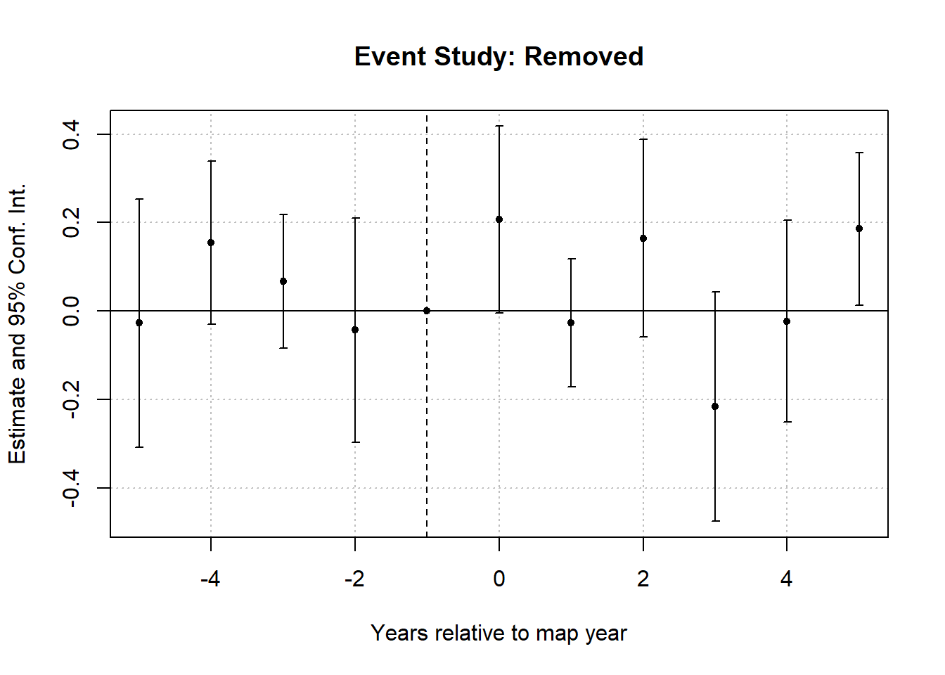
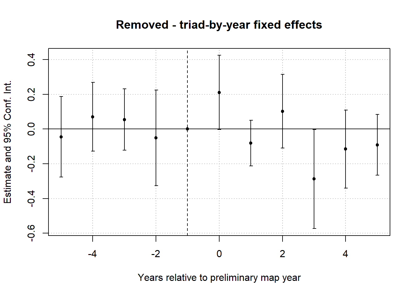
Properties removed from the preliminary SFHA are compared with always-SFHA properties. The event-time bins, omitted period, fixed effects, and clustering follow the addition specification. The plot and joint lead test provide the removal-side diagnostics discussed in Appendix A; the appropriate comparison is within this design, rather than between its coefficient levels and those of the addition design.
```{r}
# --- define sample + treatment (Removed vs Always) ----
df_es_removed <- df_prep |>
  filter(prelim_sfha_category %in% c("Removed from prelim SFHA", "Always SFHA")) |>
  mutate(treated = prelim_sfha_category == "Removed from prelim SFHA")

range(df_es_removed$sale_year, na.rm = TRUE)
# ---- event-study regression ----
mod_es_removed_none <- feols(
  log(sale_price) ~ i(event_time_binned, treated, ref = -1) | pin + sale_year,
  cluster = ~ pin10,
  data = df_es_removed
)

# ----  plot ----
iplot(mod_es_removed_none, xlab = "Years relative to map year", main = "Event Study: Removed")
```
This specification controls for common year effects but does not allow year effects to differ across North Cook, South Cook, and Chicago. The regional-control comparison below examines sensitivity to that restriction; the baseline specification alone does not establish whether regional differences explain its estimates.
```{r}
# ---- pre-trend check (leads only) ----
pretrends <- broom::tidy(mod_es_removed_none) |>
  filter(str_detect(term, "^event_time_binned::")) |>
  mutate(rel_time = as.integer(str_extract(term, "-?\\d+"))) |>
  filter(rel_time < 0) |>
  arrange(rel_time)

pretrends
# ----  joint test of pre-trends ----
wald(mod_es_removed_none, keep = "event_time_binned::-(5|4|3|2)")
```
> Read the joint test as a test that the included pretreatment coefficients are zero relative to the omitted period. It is not a test that the coefficients equal one another, and a non-significant result does not prove parallel trends.
## Extended-TWFE event profiles {#q1-etwfe-event-profiles}
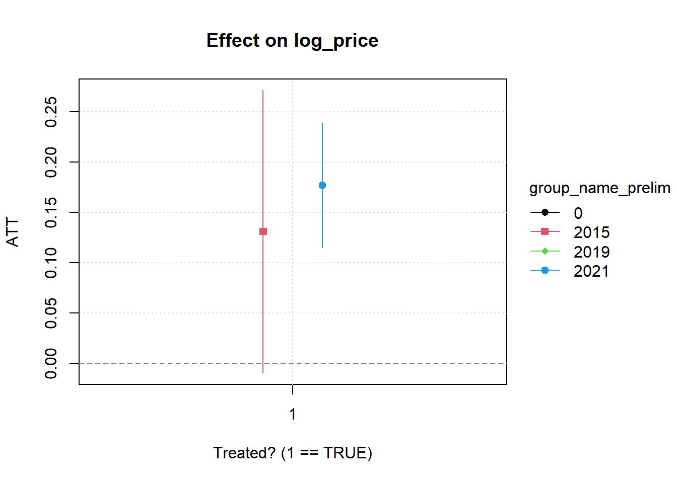
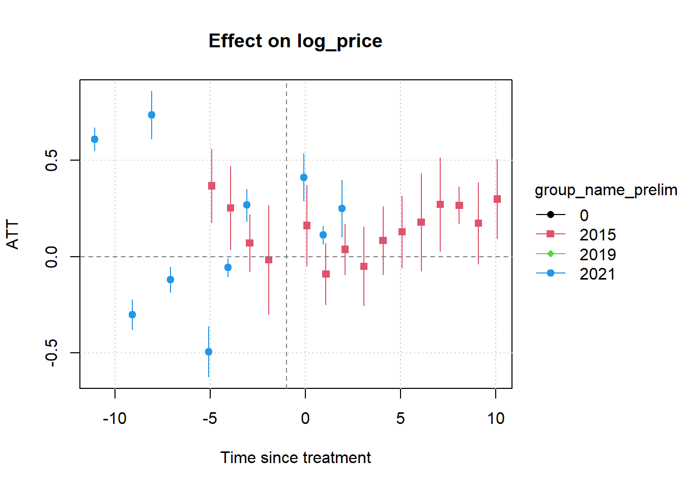
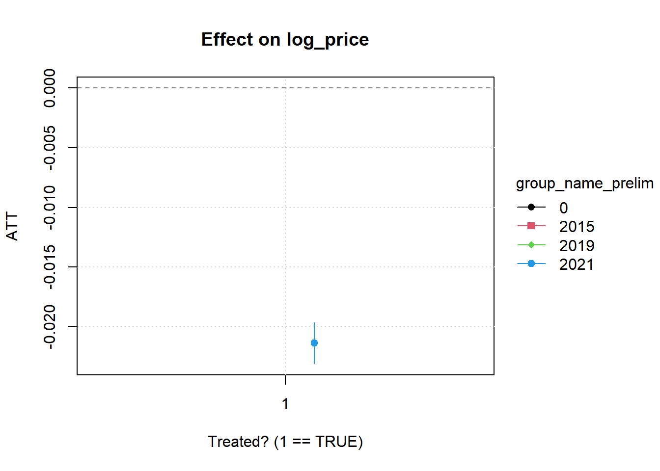
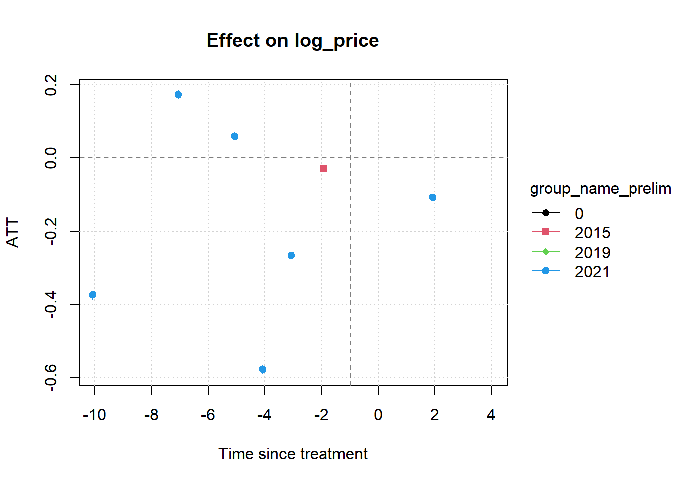
These existing extended-TWFE models produce grouped marginal effects and event profiles for preliminary-map removals, followed by additions. Each model excludes the opposite transition and uses the corresponding always-SFHA or never-SFHA comparison category. These outputs supplement the binned event studies; different estimators, aggregation, and comparison sets can produce different profiles. The earlier heading associated this output with Figure 12; an exact match to the printed figure has not been established here.
```{r}
mod2 = etwfe(
  fml = log_price ~ 1,
  tvar = sale_year,
  ivar = pin,
  xvar = group_name_prelim,
    cgroup = "never",

  gvar = treat_year_remove_prelim,
  vcov = ~pin10,
  data = (df_prep|>
            # do not want treated properties that move in opposite direction.
            filter(treat_year_add_prelim==10000 &
                     # and only want to compare to properties that were Always in the SFHA (also keeps properties that changed SFHA status),
                     change_type_prelim != "Never SFHA")
          )
  )
#mod2
emfx(mod2, type = "group")
plot(emfx(mod2), pch = c(16, 15, 18, 19))
plot(emfx(mod2, type = "event"), pch = c(16, 15, 18, 19))
```
```{r}
mod2 = etwfe(
  fml = log_price ~ 1,
  tvar = sale_year,
  ivar = pin,
  xvar = group_name_prelim,
    cgroup = "never",

  gvar = treat_year_add_prelim,
  vcov = ~pin10,
  data = (df_prep|>
            # do not want treated properties that move in opposite direction.
            filter(treat_year_remove_prelim==10000 &
                     # and only want to compare to properties that were Never in the SFHA (also keeps properties that changed SFHA status),
                     change_type_prelim != "Always SFHA")
          )
  )
#mod2
emfx(mod2, type = "group")
plot(emfx(mod2), pch = c(16, 15, 18, 19))
plot(emfx(mod2, type = "event"), pch = c(16, 15, 18, 19))
# mod2 = etwfe(
#   fml = log_price ~ 1,
#   tvar = sale_year,
#   ivar = pin,
#   xvar = group_name_prelim,
#     cgroup = "notyet",
#
#   gvar = treat_year_add_prelim,
#   vcov = ~pin10,
#   data = (df_prep|>
#             # do not want treated properties that move in opposite direction.
#             filter(treat_year_remove_prelim==10000 &
#                      # and only want to compare to properties that were Never in the SFHA (also keeps properties that changed SFHA status),
#                      change_type_prelim != "Always SFHA")
#           )
#   )
# #mod2
# emfx(mod2, type = "group")
# plot(emfx(mod2), pch = c(16, 15, 18, 19))
# plot(emfx(mod2, type = "event"), pch = c(16, 15, 18, 19))
```
## Two-year-early placebo tests {#q1-placebo-tests}
Appendix A discusses whether estimated changes appear before the preliminary map date. These placebo models move each preliminary date two years earlier, restrict observations to sales strictly before the actual preliminary date, and estimate the treated-by-placebo-period interaction with property and year fixed effects and parcel-clustered standard errors. Removals are displayed first, then additions.
A nonzero placebo estimate can reflect anticipation, differential trends, or other misspecification; it does not identify which explanation is responsible. A non-significant estimate does not rule these out. The final two tables use the actual preliminary date and the broader time window, providing a reference specification rather than additional placebo tests.
```{r}
#| label: tbl-appendixA-placebotest
#|
# df_prep must have: pin, pin10, sale_date, sale_year, pre_date, prelim_sfha_category, log_price

run_placebo_did <- function(df,
                            fake_shift_years = 2,
                            treated_label = "Added to prelim SFHA",
                            unit_fe = "pin",
                            time_fe = "sale_year",
                            cluster_var = "pin10") {
  if(treated_label == "Added to prelim SFHA"){
    df <- df |> filter(prelim_sfha_category %in% c("Added to prelim SFHA", "Never SFHA"))
  }
  if(treated_label == "Removed from prelim SFHA"){
    df <- df |> filter(prelim_sfha_category %in% c("Removed from prelim SFHA", "Always SFHA"))
  }
  df_placebo <- df |>
    mutate(
      treated = prelim_sfha_category == treated_label,
      placebo_date = pre_date %m-% years(fake_shift_years),
      placebo_post = sale_date >= placebo_date
    ) |>
    # keep only observations strictly before the *real* event (so placebo is truly placebo)
    filter(sale_date < pre_date) |>
    # optional: keep only observations with a defined placebo_date
    filter(!is.na(placebo_date))

  fml <- as.formula(paste0(
    "log_price ~ treated * placebo_post | ",
    unit_fe, " + ", time_fe
  ))

  feols(
    fml,
    cluster = as.formula(paste0("~", cluster_var)),
    data = df_placebo
  )
}


m_placebo <- run_placebo_did(bldg_sfha, treated_label = "Removed from prelim SFHA",
                             fake_shift_years = 2)
etable(m_placebo, signif.code = c("***" = .001, "**" = .01, "*" = .05, "+" = .10))
m_placebo <- run_placebo_did(bldg_sfha, treated_label = "Added to prelim SFHA",
                             fake_shift_years = 2)
etable(m_placebo, signif.code = c("***" = .001, "**" = .01, "*" = .05, "+" = .10))
```
```{r}
#| label: tbl-did_test_normal
#| tbl-cap: "Same set up as placebo test, but without the placebo. Includes all years of data."
run_normal_did <- function(df,
                            treated_label = "Added to prelim SFHA",
                            unit_fe = "pin",
                            time_fe = "sale_year",
                            cluster_var = "pin10") {
  if(treated_label == "Added to prelim SFHA"){
    df <- df |> filter(prelim_sfha_category %in% c("Added to prelim SFHA", "Never SFHA"))
  }
  if(treated_label == "Removed from prelim SFHA"){
    df <- df |> filter(prelim_sfha_category %in% c("Removed from prelim SFHA", "Always SFHA"))
  }

  df_did <- df |>
    mutate(
      treated = prelim_sfha_category == treated_label, #== treated_label,
      treated_date = pre_date,
      event_post = (sale_date >= treated_date  & pre_date_chr != "2005-01-01")
    )

  fml <- as.formula(paste0(
    "log_price ~ treated * event_post | ",
    unit_fe, " + ", time_fe
  ))

  feols(
    fml,
    cluster = as.formula(paste0("~", cluster_var)),
    data = df_did
  )
}


normal_did_add <- run_normal_did(bldg_sfha, treated_label = "Added to prelim SFHA")
etable(normal_did_add, signif.code = c("***" = .001, "**" = .01, "*" = .05, "+" = .10))
normal_did_remove <- run_normal_did(bldg_sfha, treated_label = "Removed from prelim SFHA")
etable(normal_did_remove, signif.code = c("***" = .001, "**" = .01, "*" = .05, "+" = .10))
```
## Regional controls and conditional parallel trends {#q1-conditional-trends}
Appendix A considers whether regional housing-market differences affect the Q1 comparisons. The specifications below adapt the existing triad-by-year event studies in `q1_assumption_tests.qmd` to the same addition and removal samples used above. They replace common year effects with `sale_year^Triad` while retaining property fixed effects and parcel-clustered standard errors. These are region-by-year fixed effects, not separate linear trend slopes.
The comparisons use a common complete-case sample for each treatment direction, so differences between the two specifications are not caused by missing triad identifiers. The joint tests concern the included pretreatment coefficients relative to year -1; failure to reject does not establish the unobserved post-treatment counterfactual. These tables are newly assembled from the existing specifications, not a verified reproduction of a numbered dissertation table.
```{r}
#| label: q1-conditional-trend-comparison
q1_regional_samples <- list(
  Added = df_es_add,
  Removed = df_es_removed
)
q1_regional_models <- lapply(q1_regional_samples, function(d) {
  d <- d |>
    dplyr::filter(is.finite(sale_price), sale_price > 0) |>
    tidyr::drop_na(pin, pin10, sale_year, Triad, event_time_binned, treated)
  list(
    `Common year effects` = fixest::feols(
      log(sale_price) ~ i(event_time_binned, treated, ref = -1) | pin + sale_year,
      cluster = ~pin10, data = d
    ),
    `Triad-by-year effects` = fixest::feols(
      log(sale_price) ~ i(event_time_binned, treated, ref = -1) | pin + sale_year^Triad,
      cluster = ~pin10, data = d
    )
  )
})
for (direction in names(q1_regional_models)) {
  cat("\n", direction, "to/from preliminary SFHA: coefficient comparison\n")
  print(fixest::etable(q1_regional_models[[direction]], signif.code = c("***" = .001, "**" = .01, "*" = .05, "+" = .10),
                      keep = "%event_time_binned::"))
  for (specification in names(q1_regional_models[[direction]])) {
    cat("\nJoint pretreatment test:", direction, "-", specification, "\n")
    print(fixest::wald(q1_regional_models[[direction]][[specification]],
                      keep = "event_time_binned::-(5|4|3|2)"))
  }
  fixest::iplot(q1_regional_models[[direction]][["Triad-by-year effects"]],
                xlab = "Years relative to preliminary map year",
                main = paste(direction, "- triad-by-year fixed effects"))
}
```
## Outcome transformations {#q1-outcome-transformations}
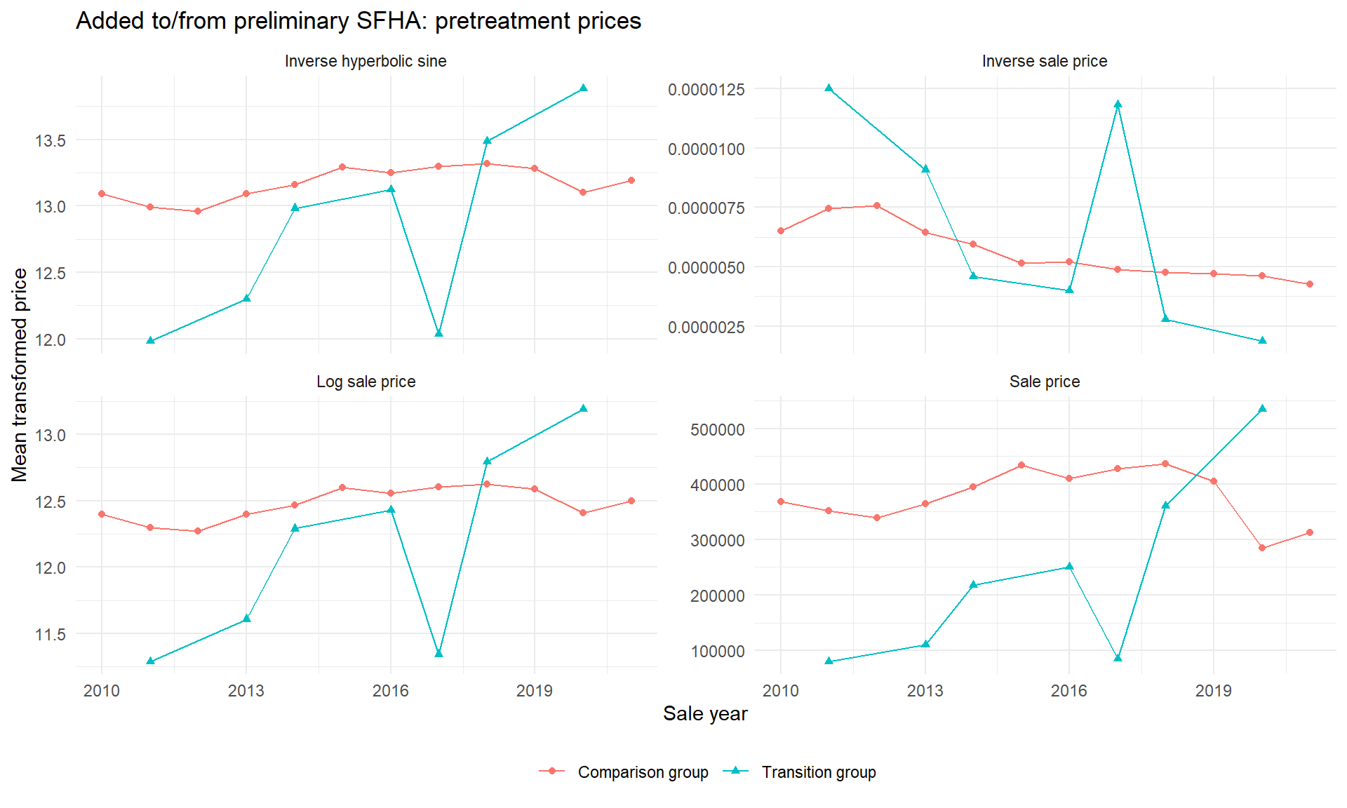
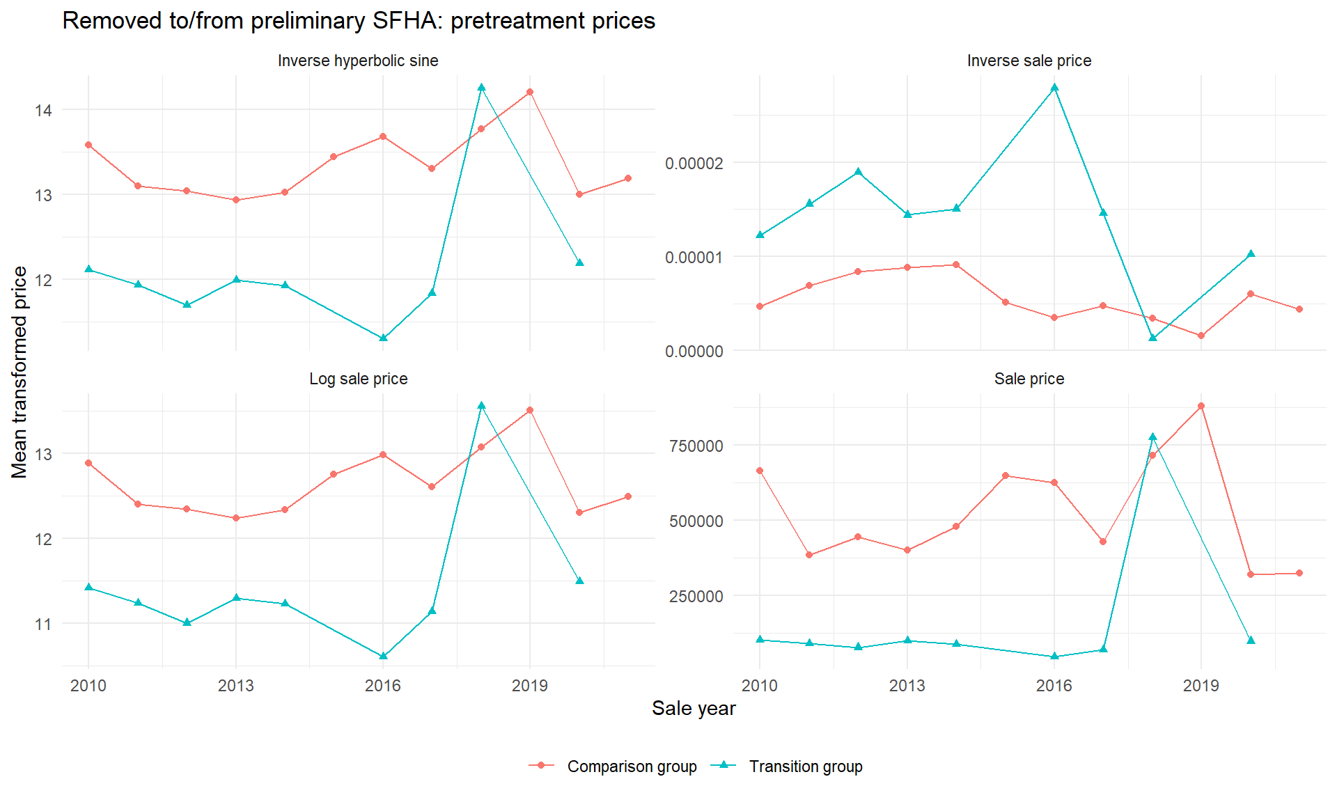
Appendix A (printed pages 95-97) discusses sale price in levels, logarithms, inverse price, and inverse hyperbolic sine. The plots below assemble all four transformations for the Q1 event-study samples. They use the same observations across transformations: finite, strictly positive prices in the pretreatment period, with addition and removal comparisons shown separately. The last two plots are supporting variations, not estimates of a new treatment effect.
Points are means of transformed sale prices by calendar year and treatment group, not transformations of the group mean. The panels use separate vertical scales. A year can pool observations from different preliminary-map cohorts, and the mix of sold properties can change over time; these descriptive plots therefore supplement the event studies rather than proving parallel trends. Inverse price is decreasing in price, so its direction must be interpreted accordingly. This newly assembled comparison is not an exact reconstruction of dissertation Figures 15-16.
```{r}
#| label: q1-transformation-comparison
#| fig-width: 10
#| fig-height: 6
q1_transformation_data <- dplyr::bind_rows(
  Added = df_es_add,
  Removed = df_es_removed,
  .id = "comparison"
) |>
  dplyr::filter(sale_date < pre_date, is.finite(sale_price), sale_price > 0) |>
  dplyr::mutate(
    group = dplyr::if_else(treated, "Transition group", "Comparison group"),
    `Sale price` = sale_price,
    `Log sale price` = log(sale_price),
    `Inverse sale price` = 1 / sale_price,
    `Inverse hyperbolic sine` = asinh(sale_price)
  )
q1_transformation_counts <- q1_transformation_data |>
  dplyr::group_by(comparison, group) |>
  dplyr::summarise(Sales = dplyr::n(), Properties = dplyr::n_distinct(pin),
                   .groups = "drop")
knitr::kable(q1_transformation_counts,
             caption = "Pretreatment observations used in each transformation")
q1_transformation_means <- q1_transformation_data |>
  dplyr::select(comparison, group, sale_year, `Sale price`, `Log sale price`,
                `Inverse sale price`, `Inverse hyperbolic sine`) |>
  tidyr::pivot_longer(cols = c(`Sale price`, `Log sale price`,
                              `Inverse sale price`, `Inverse hyperbolic sine`),
                      names_to = "transformation", values_to = "value") |>
  dplyr::group_by(comparison, group, sale_year, transformation) |>
  dplyr::summarise(mean_value = mean(value), Sales = dplyr::n(), .groups = "drop")
for (direction in c("Added", "Removed")) {
  print(ggplot2::ggplot(
    dplyr::filter(q1_transformation_means, comparison == direction),
    ggplot2::aes(sale_year, mean_value, colour = group, shape = group)
  ) + ggplot2::geom_line() + ggplot2::geom_point() +
    ggplot2::facet_wrap(~transformation, scales = "free_y", ncol = 2) +
    ggplot2::labs(title = paste(direction, "to/from preliminary SFHA: pretreatment prices"),
                  x = "Sale year", y = "Mean transformed price", colour = NULL, shape = NULL) +
    ggplot2::theme_minimal() + ggplot2::theme(legend.position = "bottom"))
}
```
## Saved distributional parallel-trends diagnostics {#q1-distributional-tests}
Appendix A (printed pages 98-99) reports distributional diagnostics associated with Roth and Sant'Anna's functional-form analysis. Existing results were located in `scripts/Q1_SFHA_DiD_test.R` and its saved `didFF` objects. The cells below display those saved results without re-estimating them or running the exploratory script.
The unlogged 2014/2022 object has a saved p-value of 0.99778, consistent with the rounded 0.998 in the dissertation. A second unlogged object has p-value 1. The saved logged-price object has p-value 0. These are different historical specifications; they should not be presented as uniformly supporting the same conclusion. The script overwrites the logged-price output during its later exploratory specification, so it is not a clean same-sample levels-versus-logs comparison. A large p-value is a failure to reject the diagnostic's null, not proof of parallel trends or of the causal interpretation.
| Saved object | Code provenance and interpretation |
|---|---|
| `didFF_Q1_model_notlogged.rds` | Uses the older parcel dataset `df_prep_land_updated_final.rds`, retains 2014 and 2022 sales, averages within property-year, and assigns the transition group to 2022. Outcome: sale price. |
| `didFF_Q1_model_out.rds` | Last written by the later logged-price specification, which assigns group 2021 using transition status and sale date relative to the preliminary date. This assignment can vary within property. |
| `didFF_model_Q1_out2.rds` | Later unlogged-price specification with the same sale-date-dependent group construction. It is distinct from the 2014/2022 comparison. |
The latter two grouping constructions require methodological review before being used as confirmatory evidence. The saved objects do not establish that these samples match the current building-based Q1 models. The historical output is shown here to make the dissertation's diagnostic evidence traceable, including the result that differs from its summary.
```{r}
#| label: q1-saved-distributional-results
#| fig-width: 9
#| fig-height: 5
q1_distribution_files <- c(
  `Sale price: 2014/2022 specification` = "outputs/didFF_Q1_model_notlogged.rds",
  `Logged price: later exploratory specification` = "outputs/didFF_Q1_model_out.rds",
  `Sale price: later exploratory specification` = "outputs/didFF_model_Q1_out2.rds"
)
q1_missing_distribution <- q1_distribution_files[!file.exists(q1_distribution_files)]
if (length(q1_missing_distribution)) {
  stop("Missing saved Q1 diagnostics: ", paste(q1_missing_distribution, collapse = ", "),
       ". Restore the saved outputs; do not substitute another specification.")
}
for (description in names(q1_distribution_files)) {
  saved_diagnostic <- readRDS(q1_distribution_files[[description]])
  if (is.null(saved_diagnostic$pval) || is.null(saved_diagnostic$plot)) {
    stop("Saved diagnostic lacks a p-value or plot: ", q1_distribution_files[[description]])
  }
  cat("\n", description, "\nSaved p-value: ", saved_diagnostic$pval, "\n", sep = "")
  print(saved_diagnostic$plot + ggplot2::labs(title = description))
  rm(saved_diagnostic)
}
```